Content from Introduction

---

Last updated on 2024-12-11 | Edit this page

Overview

Questions

• What is programming?
• How do I document code?
• How do I find reliable and safe resources or code online?

Objectives

• identify basic concepts in programming

Programming in Python

---

In most general terms, programming is the process of writing instructions for a computer. In this course we will be using Python as the language to communicate with the computer.

Strictly speaking, Python is an interpreted language, rather than a compiled language, meaning we are not communicating directly with the computer when we use Python. When we run Python code, our Python source code is first translated into byte code, which is then executed by the Python virtual machine.

Programming is a wide topic including a variety of techniques and tools. In this course we’ll be focusing on programming for statistical analysis.

IDEs

IDE stands for Integrated Development Environment. IDEs are where you will write, edit, and debug python scripts, so you want to choose one that makes you feel comfortable and includes the functionality that you need. Some open-source IDEs for Python include JupyterLab and Visual Studio Code.

Packages

Packages, or libraries, are extensions to the statistical programming language. They contain code, data, and documentation in a standardised collection format that can be installed by users, typically via a centralised software repository. A typical Python workflow will use base Python (the core operations and functions provided by your Python installation) as well as specialised data analysis and scientific packages like NumPy, SciPy and Pandas.

Best Practices

---

Let’s overview some base concepts that any programmer should always keep in mind.

Documentation

Have you ever returned to a task and tried to read a note that you quickly scrawled for yourself the last time you were working on it? Have you ever inherited a project from a colleague and found you have no idea what remains to be done?

It can be very challenging to return to your own work or a colleague’s and this goes doubly for programming. Documentation is one way we can reduce the burden on future selves and our colleagues.

Inline Documentation

As a new programmer, inline documentation can be the most helpful. Inline documentation refers to writing comments on the same line as your code. For example, if we wrote a line of code to sum 1+1, we might document it as follows:

PYTHON

1+1         # adding the numbers 1 and 1 together.

Although this is a very simple line of code and it might seem like overkill to document it in this way, these types of comments can be very helpful in jogging your memory when returning to a project. Inline comments can also help you to break multi-step programs into digestible and readable pieces.

External Documentation

Sometimes you require more detail than you can comfortably fit in your inline documentation. In this case it can be helpful to create separate files to document your project. This type of documentation will typically focus on the goals, scope, and any special instructions relating to your project rather than the details fo your code. The most common type of external documentation is a README file. It is best practice to create a basic README file for any project. A basic README should include:

• a brief description of the project,
• any special instructions for installation or use,
• the authors and any references.

README files are just text files and it is best practice is to save your README file as a README.md markdown document. This file format is automatically recognised by code repositories like GitHub, so your README contents are displayed alongside your code repository.

DocStrings

In chapter 7: functions we’ll learn about documentation specific to functions known as DocStrings.

Getting Help

---

Later on, in chapter 10: Errors and Exceptions we will cover errors in more detail. However, before we get there it’s very likely you’ll need some assistance writing Python code.

Built-in Help

There is a help function built into base Python. You can use it to investigate built-in functions, data types, and more. For example, say we want to know more about the print() function in Python:

PYTHON

help(print)

OUTPUT

Help on built-in function print in module builtins:

print(...)
    print(value, ..., sep=' ', end='\n', file=sys.stdout, flush=False)

    Prints the values to a stream, or to sys.stdout by default.
    Optional keyword arguments:
    file:  a file-like object (stream); defaults to the current sys.stdout.
    sep:   string inserted between values, default a space.
    end:   string appended after the last value, default a newline.
-- More  --

Finding Resources online

Stack Overflow is a valuable resource for programmers of all levels. It can be daunting to post your own question! Fortunately, chances are someone else has already asked a similar question!

The Official Python Documentation is another great resource.

It can also be helpful to do a general search for a particular topic or error message. It’s very likely the first few results will be from StackOverflow, followed by a few from official documentation and then you may start seeing results from personal blogs or third parties. These third party results can sometime be valuable but we should be cautious! Here are a few things to keep in mind when you are looking for online resources:

1. Don’t download or install anything unless you are certain of what it is and why you need it.
2. Don’t copy or run code unless you fully understand what it does.
3. Python is an open-source language; official documentation and resources will not be behind a paywall.
4. You may not find a resource or solution to fit your exact needs. Try to be flexible and adapt online solutions to fit your needs.

Key Points

• Python is an interpreted language.
• Code is commonly developed inside an integrated development environment.
• A typical Python workflow uses base Python and additional Python packages developed for statistical programming purposes.
• In-line and external documentation helps ensure that your code is readable.
• You can find help through the built-in help function and external resources.

Content from Python Fundamentals

---

Last updated on 2024-07-11 | Edit this page

Overview

Questions

• What basic data types can I work with in Python?
• How can I create a new variable in Python?
• How do I use a function?
• Can I change the value associated with a variable after I create it?

Objectives

• Assign values to variables.

Variables

---

Any Python interpreter can be used as a calculator:

PYTHON

3 + 5 * 4

OUTPUT

23

This is great but not very interesting. To do anything useful with data, we need to assign its value to a variable. In Python, we can assign a value to a variable, using the equals sign =. For example, we can track the weight of a patient who weighs 60 kilograms by assigning the value 60 to a variable weight_kg:

PYTHON

weight_kg = 60

From now on, whenever we use weight_kg, Python will substitute the value we assigned to it. In layperson’s terms, a variable is a name for a value.

In Python, variable names:

• can include letters, digits, and underscores
• cannot start with a digit
• are case sensitive.

This means that, for example:

• weight0 is a valid variable name, whereas 0weight is not
• weight and Weight are different variables

Types of data

---

Python knows various types of data. Three common ones are:

• integer numbers
• floating point numbers, and
• strings.

In the example above, variable weight_kg has an integer value of 60. If we want to more precisely track the weight of our patient, we can use a floating point value by executing:

PYTHON

weight_kg = 60.3

To create a string, we add single or double quotes around some text. To identify and track a patient throughout our study, we can assign each person a unique identifier by storing it in a string:

PYTHON

patient_id = '001'

Using Variables in Python

---

Once we have data stored with variable names, we can make use of it in calculations. We may want to store our patient’s weight in pounds as well as kilograms:

PYTHON

weight_lb = 2.2 * weight_kg

We might decide to add a prefix to our patient identifier:

PYTHON

patient_id = 'inflam_' + patient_id

Built-in Python functions

---

To carry out common tasks with data and variables in Python, the language provides us with several built-in functions. To display information to the screen, we use the print function:

PYTHON

print(weight_lb)
print(patient_id)

OUTPUT

132.66
inflam_001

When we want to make use of a function, referred to as calling the function, we follow its name by parentheses. The parentheses are important: if you leave them off, the function doesn’t actually run! Sometimes you will include values or variables inside the parentheses for the function to use. In the case of print, we use the parentheses to tell the function what value we want to display. We will learn more about how functions work and how to create our own in later episodes.

We can display multiple things at once using only one print call:

PYTHON

print(patient_id, 'weight in kilograms:', weight_kg)

OUTPUT

inflam_001 weight in kilograms: 60.3

We can also call a function inside of another function call. For example, Python has a built-in function called type that tells you a value’s data type:

PYTHON

print(type(60.3))
print(type(patient_id))

OUTPUT

<class 'float'>
<class 'str'>

Moreover, we can do arithmetic with variables right inside the print function:

PYTHON

print('weight in pounds:', 2.2 * weight_kg)

OUTPUT

weight in pounds: 132.66

The above command, however, did not change the value of weight_kg:

PYTHON

print(weight_kg)

OUTPUT

60.3

To change the value of the weight_kg variable, we have to assign weight_kg a new value using the equals = sign:

PYTHON

weight_kg = 65.0
print('weight in kilograms is now:', weight_kg)

OUTPUT

weight in kilograms is now: 65.0

Variables as Sticky Notes

A variable in Python is analogous to a sticky note with a name written on it: assigning a value to a variable is like putting that sticky note on a particular value.

Using this analogy, we can investigate how assigning a value to one variable does not change values of other, seemingly related, variables. For example, let’s store the subject’s weight in pounds in its own variable:

PYTHON

# There are 2.2 pounds per kilogram
weight_lb = 2.2 * weight_kg
print('weight in kilograms:', weight_kg, 'and in pounds:', weight_lb)

OUTPUT

weight in kilograms: 65.0 and in pounds: 143.0

Everything in a line of code following the ‘#’ symbol is a comment that is ignored by Python. Comments allow programmers to leave explanatory notes for other programmers or their future selves.

Similar to above, the expression 2.2 * weight_kg is evaluated to 143.0, and then this value is assigned to the variable weight_lb (i.e. the sticky note weight_lb is placed on 143.0). At this point, each variable is “stuck” to completely distinct and unrelated values.

Let’s now change weight_kg:

PYTHON

weight_kg = 100.0
print('weight in kilograms is now:', weight_kg, 'and weight in pounds is still:', weight_lb)

OUTPUT

weight in kilograms is now: 100.0 and weight in pounds is still: 143.0

Since weight_lb doesn’t “remember” where its value comes from, it is not updated when we change weight_kg.

Check Your Understanding

What values do the variables mass and age have after each of the following statements? Test your answer by executing the lines.

PYTHON

mass = 47.5
age = 122
mass = mass * 2.0
age = age - 20

Show me the solution

OUTPUT

`mass` holds a value of 47.5, `age` does not exist
`mass` still holds a value of 47.5, `age` holds a value of 122
`mass` now has a value of 95.0, `age`'s value is still 122
`mass` still has a value of 95.0, `age` now holds 102

Sorting Out References

Python allows you to assign multiple values to multiple variables in one line by separating the variables and values with commas. What does the following program print out?

PYTHON

first, second = 'Grace', 'Hopper'
third, fourth = second, first
print(third, fourth)

Show me the solution

OUTPUT

Hopper Grace

Seeing Data Types

What are the data types of the following variables?

PYTHON

planet = 'Earth'
apples = 5
distance = 10.5

Show me the solution

PYTHON

print(type(planet))
print(type(apples))
print(type(distance))

OUTPUT

<class 'str'>
<class 'int'>
<class 'float'>

Key Points

• Basic data types in Python include integers, strings, and floating-point numbers.
• Use variable = value to assign a value to a variable in order to record it in memory.
• Variables are created on demand whenever a value is assigned to them.
• Use print(something) to display the value of something.
• Use # some kind of explanation to add comments to programs.
• Built-in functions are always available to use.

Content from List and Dictionary Methods

---

Last updated on 2024-12-10 | Edit this page

Overview

Questions

• How can I store many values together?
• How can I create a list succinctly?
• How can I efficiently access nested data?

Objectives

• Identify and create lists and dictionaries
• Understand the properties and behaviours of lists and dictionaries
• Access values in lists and dictionaries
• Create and access values from nest lists and dictionaries

Values can also be stored in other Python data types such as lists, dictionaries, sets and tuples. Storing objects in a list is a fast and versatile way to apply transformations across a sequence of values. Storing objects in dictionary as key-value pairs is useful for extracting specific values i.e. performing lookup operations.

Create and access lists

---

Lists have the following properties and behaviours:

• A single list can store different primitive object types and even other lists
• Lists are ordered and have a 0-based index
• Lists can be appended to using the methods append() or insert()
• Values inside a list can be removed using the methods remove() or pop()
• Two lists can be concatenated with the operator +
• Values inside a list can be conditionally iterated through
• A list is mutable i.e. the values inside a list can be modified in place

To create a list, values are contained within square brackets i.e. [] and individually separated by commas. The function list() can also be used to create a list of values from an iterable object like a string, set or tuple.

PYTHON

# Create a list of integers using []
list_1 = [1, 3, 5, 7]
print(list_1)

OUTPUT

[1, 3, 5, 7]

PYTHON

# Unlike atomic vectors in R, a list can contain multiple primitive object types
list_2 = [1, "one", 1.0, True]
print(list_2)

OUTPUT

[1, 'one', 1.0, True]

PYTHON

# You can also use list() on an iterable object to convert it into a list
string = 'abcdefg'  
list_3 = list(string)  
print(list_3)

OUTPUT

['a', 'b', 'c', 'd', 'e', 'f', 'g']

Because lists have a 0-based index, we can access individual values by their list index position. For 0-based indexes, the first value always starts at position 0 i.e. the first element has an index of 0. Accessing multiple values by their index positions is also referred to as slicing or subsetting a list.

Note that we can use negative numbers as indices in Python. When we do so, the index -1 gives us the last element in the list, -2 gives us the second to last element in the list, and so on.

PYTHON

# Extract individual values from list_3
print('first value:', list_3[0])
print('second value:', list_3[1])
print('last value:', list_3[-1])

OUTPUT

first value: a
second value: b
last value: g

PYTHON

# A syntax quirk for slicing values is to +1 to the last value's index 
# To extract from index 0 to 2, we need to slice from [0:2+1] or [0:3]

# Extract the first three values from list_3
print('first 3 values:', list_3[0:3])

# Start from index 0 and extract values from each subsequent second position
print('every second value:', list_3[0::2])

# Start from index 1, end at index 3 and extract from each subsequent second position
print('every second value from index 1 to 3:', list_3[1:4:2])

OUTPUT

first 3 values: ['a', 'b', 'c']
every second value: ['a', 'c', 'e', 'g']
every second value from index 1 to 3: ['b', 'd']

Change list values

---

Data which can be modified in place is called mutable, while data which cannot be modified is called immutable. Strings and numbers are immutable in that when we want to change the value of a string or number variable, we can only replace the old value with a completely new value.

PYTHON

string = 'abcde'
string[0] = 'b' # Produces a type error as strings are immutable

# TypeError: 'str' object does not support item assignment

In contrast, lists are mutable and we can modify them after they have been created. We can change individual values, append new values, or reorder the whole list through sorting.

PYTHON

list_4 = ['apple', 'pear', 'plum']
print('original list_4:', list_4)

# Change the first value i.e. modify the list in place
list_4[0] = 'banana'
print('modified list_4:', list_4)

# Add new value to list using the method .insert(index number, value)
list_4.insert(1, 'apple') # Index 1 refers to the second position
print('appended list_4:', list_4)

OUTPUT

original list_4: ['apple', 'pear', 'plum']
modified list_4: ['banana', 'pear', 'plum']
appended list_4: ['banana', 'apple', 'pear', 'plum']

PYTHON

# Sorting a list also modifies it in place
list_5 = [2, 1, 3, 7]
list_5.sort()
print('list_5:', list_5)

OUTPUT

list_5: [1, 2, 3, 7]

However, be careful when modifying data in-place. If two variables refer to the same list, and you modify the list value, it will change for both variables!

PYTHON

# When we assign list_6 to list_5, it means both list_6 and list_5 point to the
# same list object, not that list_6 is a copy of list_5.  

list_6 = list_5  
print('list_5:', list_5)
print('list_6:', list_6)

# Change the first value in list_6 from 1 to 2 
list_6[0] = 2 

print('modified list_6:', list_6)
print('unmodified list_5:', list_5)

# Warning: list_5 and list_6 have both been modified in place!

OUTPUT

list_5: [1, 2, 3, 7]
list_6: [1, 2, 3, 7]
modified list_6: [2, 2, 3, 7]
unmodified list_5: [2, 2, 3, 7]

Because of this behaviour, code which modifies data in place should be handled with care. You can also avoid this behaviour by expliciting creating a copy of the original list and modifying only the object copy. This is why creating a copy of the original data object can be useful in Python.

PYTHON

list_5 = [1, 2, 3, 7]
list_7 = list_5.copy()  
print('list_5:', list_5)
print('list_7:', list_7)

# As list_7 is a completely new object copied from list_5, modifying list_7 does
# not affect list_5.  

list_7[0] = 2 
print('modified list_7:', list_7)
print('unmodified list_5:', list_5)

OUTPUT

list_5: [1, 2, 3, 7]
list_7: [1, 2, 3, 7]
modified list_7: [2, 2, 3, 7]
unmodified list_5: [1, 2, 3, 7]

Useful list functions

---

There are a lot of functions and methods which can be applied to lists, such as len(), max(), index() and so forth. Mathematical operations do not work on lists of integers, with the exception of +.

Note that + concatenates two lists into a single longer list, rather than outputting the sum of two lists of numbers.

PYTHON

list_8 = [1, 2, 3]
list_9 = [4, 5, 6]

list_8 + list_9 # This concatenates the lists and does not sum the two lists together

OUTPUT

[1, 2, 3, 4, 5, 6]

In your spare time after this workshop, you can search for different list functions and methods and test them out yourselves.

Nested lists

---

We have previously mentioned that lists can be used to store other Python object types, including lists. This means that we can create nested lists in Python i.e. lists containing lists containing values. This property is useful when we have a collection of values that we want to access or transform as a subgroup.

To create a nested list, we also use [] or list() to contain one or more lists of values of interest.

PYTHON

veg_stock = [
    ['lettuce', 'lettuce', 'tomato', 'zucchini'],
    ['lettuce', 'lettuce', 'carrot', 'zucchini'],
    ['lettuce', 'basil', 'tomato', 'zucchini']
    ]

# Check that veg_stock is a list object
print(type(veg_stock))

# Check that the first value in veg_stock is itself a list
print(veg_stock[0], 'has type', type(veg_stock[0]))  

OUTPUT

<class 'list'>
['lettuce', 'lettuce', 'tomato', 'zucchini'] has type <class 'list'>

To extract the first sub-list within the veg_stock list object, we refer to its index like we would with any other value inside a list i.e. veg_stock[1] points to the second sub-list within the veg_stock list.

To access an individual string value inside a sub-list, we make use of a second index, which points to an individual value inside the sub-list.

PYTHON

print(veg_stock[0]) # Access the first sub-list 
print(veg_stock[0][0]) # Access the first value in the first sub-list 

print(type(veg_stock[0])) # The first value in veg_stock is a list
print(type(veg_stock[0][0])) # The first value in the first list in veg_stock is a string

OUTPUT

['lettuce', 'lettuce', 'tomato', 'zucchini']
lettuce
<class 'list'>
<class 'str'>

In general, however, when we are analysing a large collection of values, the best practice is to structure those values in columns and rows as a tabular Pandas data frame object. This is covered in another Carpentries Course called Python for Social Sciences.

Lists are still incredibly versatile and useful when you have a collection of values that need to be efficiently accessed or transformed. For example, data frame column names are commonly extracted and stored inside a list, so that the same transformation can then be mapped across multiple columns.

Create and access dictionaries

---

A dictionary is a Python data type that is particularly suited for enabling quick lookup operations on unstructured data sets.

A dictionary can therefore be thought of as an unordered list where every item or value is associated with a unique key (i.e. a self-defined index of unique strings or numbers). The index values are called keys and a dictionary contains key-value pairs with the format {key: value(s)}.

Dictionaries can be created by listing individual key-values pairs inside {} or using dict().

PYTHON

# A key-value pair can contain single or multiple values  
# Keys are treated as case sensitive and unique
# Multiple values are first stored inside a list  

teams = {
    'data science': ['Mei Ling', 'Paul', 'Gwen', 'Suresh'],
    'user design': ['Amy', 'Linh', 'Sasha'],
    'software dev': ['David', 'Prya'],
    'comms': 'Taylor' 
    } 

When using dict(), we need to indicate which key is associated with which value. This can be done directly using tuples, direct association i.e. using = or using zip(), which creates a set of tuples from an iterable list.

PYTHON

# To use dict(), key-value pairs are can be stored inside tuples  
ds_emp_status = dict([
        ('Mei Ling', 'full time'),
        ('Paul', 'full time'),
        ('Gwen', 'part time'),
        ('Suresh', 'part time')
    ])  

# Key-value pairs can also be assigned by direct association  
# Keys cannot be strings i.e. wrapped in '' using this approach
ud_emp_status = dict(
    Amy = 'full time',
    Linh = 'full time',
    Sasha = 'casual' 
    ) 

# zip() can also be used if each key has only one value  
sd_emp_status = dict(zip(
    ['David', 'Prya'],
    ['full time', 'full time']
    ))

To access a specific value inside a dictionary, we need to specify its key using []. This is similar to slicing or subsetting a list by specifying its index using [].

PYTHON

# Access the values associated with the key 'data science'
print(teams['data science'])

print('The object teams is of type', type(teams))
print('The dict value', teams['data science'], 'is of type', type(teams['data science']))

OUTPUT

['Mei Ling', 'Paul', 'Gwen', 'Suresh']
The data object teams is of type <class 'dict'>
The value ['Mei Ling', 'Paul', 'Gwen', 'Suresh'] is of type <class 'list'>

We can also access a value from a dictionary using the get() method.

PYTHON

print(teams.get('user design'))

# get() also enables us to return an alternate string when the key is not found   
# This prevents our code from returning an error message that halts the analysis

print(teams.get('data engineering', 'WARNING: key does not exist'))

OUTPUT

['Amy', 'Linh', 'Sasha']
WARNING: key does not exist

To access data inside a dictionary, we can also perform the following other actions:

• Check whether a key exists in a dictionary using the keyword in
• Retrieve unique dictionary keys using dict.keys()
• Retrieve dictionary values using dict.values()
• Retrieve dictionary items using dict.items()

PYTHON

# Check whether a key exists in a dictionary 
print('data science' in teams) 
print('Data Science' in teams) # Keys are case sensitive  

# Retrieve all dictionary keys  
print(teams.keys())
print(sd_emp_status.keys())

# Retrieve all dictionary values  
print(sd_emp_status.values())  

# Retrieve all dictionary key-value pairs
print(sd_emp_status.items())

OUTPUT

True
False
dict_keys(['data science', 'user design', 'software dev', 'comms'])
dict_keys(['David', 'Prya'])
dict_values(['full time', 'full time'])
dict_items([('David', 'full time'), ('Prya', 'full time')])

To add a new key-value pair to an existing dictionary, we can create a new key and directly attach a new value to it using = or alternatively use the method update().

PYTHON

print('original dict items:', sd_emp_status.items())  

# Add new key-value pair using direct assignment  
sd_emp_status['Mohammad'] = 'full time'

# Add new key-value pair using update({'key': 'value'})   
sd_emp_status.update({'Carrie': 'part time'})

print('updated dict items:', sd_emp_status.items())    

OUTPUT

original dict items: dict_items([('David', 'full time'), ('Prya', 'full time')])
updated dict items: dict_items([('David', 'full time'), ('Prya', 'full time'),
('Mohammad', 'full time'), ('Carrie', 'part time')])

Because keys are unique, a dictionary cannot contain two keys with the same name. This means that adding an item using a key that is already present in the dictionary will cause the previous value to be overwritten.

PYTHON

print('original dict items:', sd_emp_status.items())  

# As the key 'Carrie' already exists, its value will be overwritten
sd_emp_status['Carrie'] = 'full time'
print('updated dict items:', sd_emp_status.items())  

OUTPUT

original dict items: dict_items([('David', 'full time'), ('Prya', 'full time'),
('Mohammad', 'full time'), ('Carrie', 'part time')])
updated dict items: dict_items([('David', 'full time'), ('Prya', 'full time'),
('Mohammad', 'full time'), ('Carrie', 'full time')])

To remove a key-value pair for an existing dictionary, we can use the del keyword or the method pop(). Using pop() also enables us to return an alternate string if we trt to remove a non-existing key, which prevents our code from returning an error message that halts the analysis.

PYTHON

print('original dict items:', sd_emp_status.items())

# Delete dictionary keys using del and pop()
del sd_emp_status['Mohammad']
sd_emp_status.pop('Carrie')
sd_emp_status.pop('Anuradha', 'WARNING: key does not exist') # Does not generate an error

print('modified dict items:', sd_emp_status.items())  

OUTPUT

original dict items: dict_items([('David', 'full time'), ('Prya', 'full time'),
('Mohammad', 'full time'), ('Carrie', 'full time')])
modified dict items: dict_items([('David', 'full time'), ('Prya', 'full time')])

Nested dictionaries

---

Similar to lists, dictionaries can be nested as we can also store dictionaries as values inside a key-value pair using {}. Nested dictionaries are useful when we need to store unstructured data in a complex structure. For example, JSON data is commonly used for transmitting data in web applications and often exists in a nested structure that can be stored using nested dictionaries in Python.

PYTHON

# Individual dictionaries are enclosed in {} and separated by a comma
nested_dict = {
    'dict_1': { # First key is a dictionary of key-value pairs 
        'key_1a': 'value_1a',
        'key_1b': 'value_1b'
                },
    'dict_2': { # Second key is another dictionary of key-value pairs
        'key_2a': 'value_2a',
        'key_2b': 'value_2b'
                }
            }

print(nested_dict)

OUTPUT

{'dict_1': {'key_1a': 'value_1a', 'key_1b': 'value_1b'},
 'dict_2': {'key_2a': 'value_2a', 'key_2b': 'value_2b'}}

Similar to working with nested lists, to extract a value from the first sub-dictionary, we specify both the main dictionary and sub-dictionary keys using [].

PYTHON

# Extract the value for key 2a in dict_2
print('original value:', nested_dict['dict_2']['key_2a'])

# Adding or updating a value can be done through the same approach
nested_dict['dict_2']['key_2a'] = "modified_value_2a"  

print('modified value:', nested_dict['dict_2']['key_2a'])

OUTPUT

original value: value_2a
modified value: modified_value_2a

Optional: converting lists and dictionaries to Pandas data frames

---

Lists and dictionaries can be easily converted into a tabular Pandas data frame format. This can be useful when you need to create a small data set for unit testing purposes.

PYTHON

# Import pandas library
import pandas as pd

# Create a dictionary with each key-value pair representing a data frame column
data = {
    'col_1': [3, 2, 1, 0],
    'col_2': ['a', 'b', 'c', 'd']
    }

df = pd.DataFrame.from_dict(data) 

print(df) # Outputs data as a tabular Pandas data frame   
print(type(df))

OUTPUT

   col_1 col_2
0      3     a
1      2     b
2      1     c
3      0     d
<class 'pandas.core.frame.DataFrame'>

Key Points

• Lists can contain any Python object including other lists
• Lists are ordered i.e. indexed and can therefore be sliced by index number
• Unlike strings and integers, the values inside a list can be modified in place
• A list which contains other lists is referred to as a nested list
• Dictionaries behave like unordered lists and are defined using key-value pairs
• Dictionary keys are unique
• A dictionary which contains other dictionaries is referred to as a nested dictionary
• Values inside nested lists and dictionaries can be accessed by an additional index

Content from Data Transformation

---

Last updated on 2024-12-11 | Edit this page

Overview

Questions

• How can I process tabular data files in Python?

Objectives

• Explain what a library is and what libraries are used for.
• Import a Python library and use the functions it contains.
• Read tabular data from a file into a program.
• Clean and prepare data.
• Merge and reshape data.
• Handle missing values.
• Aggregate and summarize data.

Introduction

---

What is a Package/Library in Python?

In Python, a library (or package) is a collection of pre-written code that you can use to perform common tasks without needing to write the code from scratch. It’s a toolbox that provides tools (functions, classes, and modules) to help you solve specific problems.

Python packages save time and effort by providing solutions to common programming challenges. Instead of reinventing the wheel, you can import these tools into your scripts and use them to complete tasks more easily.

A Python package for data manipulations: pandas

In this lesson, we will focus on using the pandas library in Python to perform common data wrangling tasks.

pandas is an open-source Python library for data manipulation and analysis. It provides data structures like DataFrame and Series that make it easy to handle and analyze data.

Series

A Series is a one-dimensional labeled array, similar to a list. It can hold any data type, such as integers, strings, or even more complex data types.

Key Features:

• It’s one-dimensional, so it holds data in a single column.
• It has an index (labels) that you can use to access specific elements.
• Each element in the Series has a label (index) and a value.

Example of a Series:

PYTHON

import pandas as pd

# Create a Series from a list

data = [10, 20, 30, 40, 50]
series = pd.Series(data)

# Print the Series

print(series)

Output:

OUTPUT

0 10
1 20
2 30
3 40
4 50
dtype: int64

The index is 0, 1, 2, 3, 4, and the values are 10, 20, 30, 40, 50. pandas automatically creates an index for you (starting from 0), but you can also specify a custom index.

DataFrame

A DataFrame is a two-dimensional, table-like structure (similar to a spreadsheet or SQL table) that can hold multiple Series. It is the most commonly used pandas object.

A DataFrame consists of:

• Rows (with an index, just like a Series),
• Columns (which are each Series).

You can think of a DataFrame as a collection of Series that share the same index.

Key Features:

• It’s two-dimensional.
• Each column is a Series.
• It has both row and column labels (indexes and column names).
• It can hold multiple data types (integers, strings, floats, etc.).

Example of a DataFrame:

PYTHON

import pandas as pd

# Create a DataFrame using a dictionary

data = {
'Name': ['Alice', 'Bob', 'Charlie'],
'Age': [25, 30, 35],
'City': ['New York', 'Paris', 'Seoul']
}
df = pd.DataFrame(data)

# Print the DataFrame

print(df)

Output:

OUTPUT

Name Age City
0 Alice 25 New York
1 Bob 30 Los Angeles
2 Charlie 35 Chicago

• The rows are indexed from 0, 1, 2 (default index).
• The columns are Name, Age, and City.
• Each column is a Series, so the Name column is a Series, the Age column is another Series, etc.

Import methods

In Python, libraries (or modules) can be imported into your code using the import statement. This allows you to access the functions, classes, and methods defined in that library. There are several ways to do it:

1. Full import: import pandas

• Use with pandas.DataFrame(), pandas.Series(), etc.

2. Import with alias: import pandas as pd

• Use with pd.DataFrame(), pd.Series(), etc.

3. Import specific functions or classes: from pandas import DataFrame

• Use directly as DataFrame().

4. Import multiple specific elements: from pandas import DataFrame, Series

In general, we use the option 2 for pandas.

Loading data

---

Loading CSV data

You can load a CSV file into a pandas DataFrame using the read_csv() function:

PYTHON

df = pd.read_csv('path\to\file.csv')
print(df.head())

• read_csv() reads the CSV file located at path\to\file.csv and loads it into a pandas DataFrame (df).
• By default, it assumes that the file has a header row (i.e., column names) in the first row.

If the file does not have a header, you can use the header=None parameter to let pandas generate default column names.

PYTHON

df = pd.read_csv('path\to\file.csv', header=None)

You can pass arguments like sep if the file uses a different delimiter (e.g., tab-separated \t).

PYTHON

df = pd.read_csv('path\to\file.csv', sep=`t`)

Raw string literal

In Python, the r prefix before a string is used to create a raw string literal. This tells Python to treat the string exactly as it is, without interpreting backslashes (\) as escape characters.

PYTHON

df = pd.read_csv(r'path\to\file.csv')

In regular strings, backslashes are used as escape characters. For example, \n represents a new line.

Loading Excel data

pandas provides the read_excel() function for reading Excel files.

PYTHON

df = pd.read_excel('path\to\file.xlsx')

You can specify the sheet name if the file contains multiple sheets. By default, it will load the first sheet.

PYTHON

df = pd.read_excel('data\sales_data.xlsx', sheet_name='Q1_2024')

You can also load multiple sheets into a dictionary of DataFrames using sheet_name=None.

PYTHON

df = pd.read_excel('data\sales_data.xlsx', sheet_name=None)

Other file formats

You can also load data from other formats like JSON, or SQL databases:

• JSON: pd.read_json('your_file.json')
• SQL: pd.read_sql('SELECT * FROM table', connection)

Data exploration

---

Viewing the first few rows

PYTHON

print(df.head())  # Shows the first 5 rows

If you want to see more (or fewer) rows, you can pass a number to head(), such as df.head(10) to view the first 10 rows.

Similarly, you can use the tail() method to view the last few rows of the DataFrame.

Viewing the columns

PYTHON

print(df.columns)  # Shows the first 5 rows

Unique values in columns

To get a sense of the distinct values in a column, the unique() and value_counts() methods are useful.

PYTHON

df['column_name'].unique()

The unique() method shows all the unique values in a column.

PYTHON

df['column_name'].value_counts()

The value_counts() method returns the count of unique values in the column, sorted in descending order. This is particularly useful for categorical data.

Checking for missing values

The isnull() method returns a DataFrame of the same shape as df, where each element is a boolean (True for missing values and False for non-missing values).

PYTHON

print(df.isnull())

To get the total number of missing values in each column, you can chain sum() to isnull().

PYTHON

print(df.isnull().sum())

This gives you a count of how many missing values are present in each column.

Summary statistics

To get a quick overview of the numerical data, you can use:

PYTHON

print(df.describe())

The describe() method provides summary statistics for all numeric columns, including:

• count: the number of non-null entries
• mean: the average value
• std: the standard deviation
• min/max: the minimum and maximum values
• 25%, 50%, 75%: the percentiles

Checking the data types

To understand the types of data in each column:

PYTHON

print(df.dtypes)

Exploring a SDMX dataset

Using the education.csv dataset in the materials for this episode, write the lines of code to:

• Import pandas
• Load the dataset into a pandas DataFrame
• Print the list of columns in this dataset
• Print the unique values of the REF_AREA column

Show me the solution

PYTHON

import pandas as pd

df = pd.read_csv(r"education.csv")

print(df.columns)
print(df["REF_AREA"].unique())

OUTPUT

Index(['STRUCTURE', 'STRUCTURE_ID', 'STRUCTURE_NAME', 'ACTION', 'REF_AREA',
       'Reference area', 'MEASURE', 'Measure', 'UNIT_MEASURE',
       'Unit of measure', 'INST_TYPE_EDU', 'Type of educational institution',
       'EDUCATION_LEV', 'Education level', 'AGE', 'Age', 'SUBJ_TYPE',
       'Subject', 'OBS_VALUE', 'Observation value', 'OBS_STATUS',
       'Observation status', 'UNIT_MULT', 'Unit multiplier',
       'STATISTICAL_OPERATION', 'Statistical operation', 'REF_PERIOD',
       'Reference period', 'DECIMALS', 'Decimals'],
      dtype='object')
['BFR' 'CHN' 'ESP' 'ISL' 'MEX' 'CHE' 'DEU' 'LTU' 'SAU' 'AUS' 'CAN' 'NLD'
 'CHL' 'FRA' 'KOR' 'GRC' 'LUX' 'ROU' 'FIN' 'IND' 'IRL' 'ISR' 'CZE' 'SVK'
 'TUR' 'USA' 'SVN' 'BGR' 'SWE' 'ZAF' 'UKM' 'NZL' 'OECD' 'BFL' 'IDN' 'NOR'
 'DNK' 'HRV' 'HUN' 'ARG' 'CRI' 'EST' 'COL' 'PER' 'POL' 'PRT' 'UKB' 'ITA'
 'BRA' 'JPN' 'LVA' 'EU25' 'G20' 'AUT']

Cleaning data

---

Renaming columns

You may want to rename columns for clarity:

PYTHON

df.rename(columns={'old_name': 'new_name'}, inplace=True)

Callout

The inplace=True parameter means that we are modifying the original DataFrame df directly.

By default, inplace=False, which means the following line won’t rename the old_name column:

PYTHON

df.rename(columns={'old_name': 'new_name'})

An alternative is to create a new DataFrame with the renamed columns and assign it back to df:

PYTHON

df = df.rename(columns={'old_name': 'new_name'})

The inplace parameter is present in many other pandas methods.

Dropping columns

If you no longer need a column, you can drop it:

PYTHON

df.drop(columns=['column_name'], inplace=True)

You can also select specific columns from a DataFrame by passing a list of column names to the DataFrame inside double brackets.

PYTHON

df = df[["col1", "col2"]]

Removing duplicates

To remove duplicate rows, use the drop_duplicates() method, which removes all duplicate rows by default.

PYTHON

df_cleaned = df.drop_duplicates()

You can also specify which columns to check for duplicates by passing a subset to the subset parameter:

PYTHON

df_cleaned = df.drop_duplicates(subset=['A'])

This will remove duplicates based only on column A.

Handling missing data

You can handle missing data it in various ways:

• Dropping rows with missing values:

PYTHON

df.dropna(inplace=True)

• Filling missing values with a default value:

PYTHON

df.fillna(0, inplace=True)  # Fill missing values with 0

Callout

Some methods, such as fillna() can be applied both on Series and DataFrame objects.

PYTHON

df['A'] = df['A'].fillna(0) # Fill missing values in column 'A' with 0

First cleaning steps

Using the education.csv dataset in the materials for this episode (continuing on the script of the previous exercise), write the lines of code to:

• Keep only the following columns: REF_AREA, AGE, SUBJ_TYPE, OBS_VALUE, REF_PERIOD
• Rename them with simpler names: iso3, age, subject, value, year
• Drop rows with missing data

Show me the solution

PYTHON

# Keeping only the necessary columns
df = df[["REF_AREA", "AGE", "SUBJ_TYPE", "OBS_VALUE", "REF_PERIOD"]]

# Rename them
df.rename(columns={
    "REF_AREA": "iso3",
    "AGE": "age",
     "SUBJ_TYPE": "subject",
     "OBS_VALUE": "value",
     "REF_PERIOD": "year"},
     inplace=True)

# Drop rows with missing data
df.dropna(inplace=True)

Transforming data

---

Filtering rows

You can filter rows based on certain conditions. For example, to filter for rows where the column age is greater than 30:

PYTHON

df_filtered = df[df['age'] > 30]

Another way to do this is to use loc (Label Based Indexing):

PYTHON

df_filtered = df.loc[df['age'] > 30]

Replacing values based on condition

loc can also be used to replace values in a DataFrame based on conditions. Let’s assume we have the following DataFrame, and we want to update certain values based on specific conditions.

PYTHON

data = {
    'Name': ['Alice', 'Bob', 'Charlie', 'David'],
    'Age': [25, 30, 35, 40],
    'City': ['New York', 'Los Angeles', 'Chicago', 'San Francisco']
}

df = pd.DataFrame(data)
print("Original DataFrame:")
print(df)

OUTPUT

Original DataFrame:
      Name  Age             City
0    Alice   25         New York
1      Bob   30    Los Angeles
2  Charlie   35          Chicago
3    David   40  San Francisco

Suppose we want to replace the city for anyone over the age of 30 with Seattle.

PYTHON

# Replace 'City' with 'Seattle' where 'Age' is greater than 30
df.loc[df['Age'] > 30, 'City'] = 'Seattle'

print("\nUpdated DataFrame:")
print(df)

OUTPUT

Updated DataFrame:
      Name  Age      City
0    Alice   25  New York
1      Bob   30  Los Angeles
2  Charlie   35   Seattle
3    David   40   Seattle

• df['Age'] > 30: This is the condition used to filter rows where the Age is greater than 30.
• df.loc[df['Age'] > 30, 'City']: This selects the City column for those rows where the condition is true.
• = 'Seattle': This replaces the value in the City column with ‘Seattle’ for those rows.

Sorting data

To sort your DataFrame by a specific column:

PYTHON

df_sorted = df.sort_values(by='column_name', ascending=False)

Creating new columns

You can create new columns based on existing ones. For example:

PYTHON

df['new_column'] = df['column1'] + df['column2']

Replace values using map

The map() method in pandas allows you to apply a mapping or a function to each element in the Series. You can use map() with a dictionary to replace values in a Series according to the mapping provided.

PYTHON

data = {
    'Name': ['Alice', 'Bob', 'Charlie', 'David'],
    'City': ['NY', 'LA', 'CHI', 'SF']
    }

df = pd.DataFrame(data)

# Create a dictionary for mapping

city_map = {
    'NY': 'New York',
    'LA': 'Los Angeles',
    'CHI': 'Chicago',
    'SF': 'San Francisco'
    }

# Apply the map function to replace city abbreviations

df['City'] = df['City'].map(city_map)

print(df)

OUTPUT

Name City
0 Alice New York
1 Bob Los Angeles
2 Charlie Chicago
3 David San Francisco

• city_map is a dictionary where the keys are the city abbreviations and the values are the full city names.
• df['City'].map(city_map): This replaces the city abbreviations with the corresponding full city names from the city_map dictionary.

Selection and mapping

We are still using the education.csv dataset in the materials for this episode (continuing on the script of the previous exercise).

• Now, we would like to focus on a subset of education subjects, instead of using the full list (17 subjects). Write the lines of code to select only the 8 subjects listed below.

You can use the isin() method in pandas is used to filter rows .

• You may have noticed that the column for subjects labels in the raw data was filled with missing values. For a better readability, we will transform subject codes into labels, using the following mapping:
  • READ: “Reading, writing and literature”
  • MATH: “Mathematics”
  • NSCI: “Natural sciences”
  • SSCI: “Social sciences”
  • SLAN: “Second language”
  • OLAN: “Other languages”
  • PHED: “Physical education and health”
  • ARTS: “Arts”

Show me the solution

PYTHON

# Selecting only the 8 main subjects and assign to a new dataframe
df_subset = df.loc[df['subject'].isin(["READ", "MATH", "NSCI", "SSCI", "SLAN", "OLAN", "PHED", "ARTS"])]

# Adding labels
df_subset["subject_label"] = df_subset["subject"].map({
    "READ": "Reading, writing and literature",
    "MATH": "Mathematics",
    "NSCI": "Natural sciences",
    "SSCI": "Social sciences",
    "SLAN": "Second language",
    "OLAN": "Other languages",
    "PHED": "Physical education and health",
    "ARTS": "Arts"})

Pivoting data

Pivoting and melting are two important operations for reshaping data in pandas. They are used to transform a DataFrame from “long” format to “wide” format, and vice versa.

Pivot

The pivot() method reshapes the data by turning unique values from one column into new columns. It’s useful when you want to convert a “long” format DataFrame (where each row represents a single observation) into a “wide” format (where each unique value becomes a column).

PYTHON

data = {
    'Date': ['2021-01-01', '2021-01-01', '2021-01-02', '2021-01-02'],
    'City': ['New York', 'Los Angeles', 'New York', 'Los Angeles'],
    'Temperature': [30, 75, 32, 77],
}

df = pd.DataFrame(data)

# Pivoting the data
pivot_df = df.pivot(index='Date', columns='City', values='Temperature')
print(pivot_df)

OUTPUT

City            Los Angeles  New York
Date
2021-01-01            75        30
2021-01-02            77        32

• The Date column is used as the index.
• The City column values are turned into new columns.
• The Temperature column is used to populate the new DataFrame.

Melt

The melt() function is the opposite of pivot(). It transforms a DataFrame from wide format to long format.

PYTHON

data = {
    'Date': ['2021-01-01', '2021-01-02'],
    'New York': [30, 32],
    'Los Angeles': [75, 77],
}

df = pd.DataFrame(data)

# Melting the data
melted_df = df.melt(id_vars=['Date'], var_name='City', value_name='Temperature')
print(melted_df)

OUTPUT

         Date           City  Temperature
0  2021-01-01       New York           30
1  2021-01-02       New York           32
2  2021-01-01  Los Angeles           75
3  2021-01-02  Los Angeles           77

• The Date column remains fixed (as id_vars).
• The New York and Los Angeles columns are melted into a single City column, with corresponding values in the Temperature column.

Pivot method

You are given a dataset containing sales information for different products over a few months.

PYTHON

import pandas as pd

# Create the DataFrame
data = {
    'Product': ['A', 'A', 'A', 'B', 'B', 'B', 'C', 'C', 'C'],
    'Month': ['January', 'February', 'March', 'January', 'February', 'March', 'January', 'February', 'March'],
    'Sales': [100, 150, 200, 80, 120, 160, 130, 170, 220]
}

df = pd.DataFrame(data)

Use the pivot() method to rearrange this DataFrame so that the months become columns, and each product’s sales data for each month appears under its respective column.

Show me the solution

PYTHON

pivot_df = df.pivot(index='Product', columns='Month', values='Sales')

Merging and joining data

---

Merging DataFrames

The merge() function in pandas is used to combine two DataFrames based on one or more common columns. It’s similar to SQL joins.

The basic syntax for merging two DataFrames is:

PYTHON

pd.merge(left, right, how='inner', on=None, left_on=None, right_on=None)

• left: The first DataFrame.
• right: The second DataFrame.
• how: The type of merge to perform. Options include:
  • left: Use only keys from the left DataFrame (like a left join in SQL).
  • right: Use only keys from the right DataFrame (like a right join in SQL).
  • outer: Use keys from both DataFrames, filling in missing values with NaN (like a full outer join in SQL).
  • inner: Use only the common keys (like an inner join in SQL, default option).
• on: The column or index level names to join on. If not specified, it will join on columns with the same name in both DataFrames.
• left_on and right_on: Specify columns from left and right DataFrames to merge on if the column names are different.

In the following example, we merge DataFrames on multiple columns by passing a list to the on parameter.

PYTHON

df1 = pd.DataFrame({
    'Name': ['John', 'Anna', 'Peter'],
    'City': ['NY', 'LA', 'SF'],
    'Age': [22, 25, 28]
})

df2 = pd.DataFrame({
    'Name': ['John', 'Anna', 'Peter'],
    'City': ['NY', 'LA', 'DC'],
    'Salary': [50000, 60000, 70000]
})

# Merge on multiple columns
merged_df = pd.merge(df1, df2, how='inner', on=['Name', 'City'])
print(merged_df)

OUTPUT

    Name City  Age  Salary
0   John   NY   22   50000
1   Anna   LA   25   60000

Concatenating DataFrames

In addition to merging DataFrames, pandas provides the concat() function, which is useful for combining DataFrames along a particular axis (either rows or columns). While merge() is typically used for combining DataFrames based on a shared key or index, concat() is more straightforward and is generally used when you want to append or stack DataFrames together.

The basic syntax for concat() is:

PYTHON

pd.concat([df1, df2], axis=0, ignore_index=False, join='outer')

• [df1, df2]: A list of DataFrames to concatenate.

• axis: The axis along which to concatenate:

  • axis=0: Concatenate along rows (default behavior). This stacks DataFrames on top of each other.
  • axis=1: Concatenate along columns, aligning DataFrames side-by-side.

• ignore_index: If True, the index will be reset (i.e., it will generate a new index). If False, the original indices of the DataFrames are preserved.

• join: Determines how to handle indices (or columns when axis=1):

  • outer: Takes the union of the indices (or columns) from both DataFrames (default).
  • inner: Takes the intersection of the indices (or columns), excluding any non-overlapping indices (or columns).

When concatenating along rows (which is the default behavior), the DataFrames are stacked on top of each other, and the rows are added to the end of the previous DataFrame. This is commonly used to combine datasets with the same structure but with different data.

Here is an example for concatenating DataFrames with the same columns:

PYTHON

df1 = pd.DataFrame({
    'ID': [1, 2, 3],
    'Name': ['John', 'Anna', 'Peter']
})

df2 = pd.DataFrame({
    'ID': [4, 5],
    'Name': ['Linda', 'James']
})

# Concatenate along rows (stack vertically)
concatenated_df = pd.concat([df1, df2], axis=0, ignore_index=True)
print(concatenated_df)

OUTPUT

   ID   Name
0   1   John
1   2   Anna
2   3  Peter
3   4  Linda
4   5  James

In this case:

• The two DataFrames df1 and df2 are stacked vertically.
• The ignore_index=True parameter ensures that the index is reset to a default integer index (0 to 4).
• If you didn’t set ignore_index=True, the original indices from df1 and df2 would be preserved.

Merging datasets

We are given two datasets: one containing employee details and the other containing their department information. We want to merge these two datasets on the common column Employee_ID to create a single DataFrame that contains employee details with their department names, while making sure we won’t drop any observation.

PYTHON

import pandas as pd

# Create the Employee DataFrame
employee_data = {
    'Employee_ID': [101, 102, 103, 104, 105],
    'Employee_Name': ['Alice', 'Bob', 'Charlie', 'David', 'Eva'],
    'Age': [25, 30, 35, 40, 45]
}

employee_df = pd.DataFrame(employee_data)

# Create the Department DataFrame
department_data = {
    'Employee_ID': [101, 102, 103, 106],
    'Department': ['HR', 'Finance', 'IT', 'Marketing']
}

department_df = pd.DataFrame(department_data)

# Display both DataFrames
print("Employee DataFrame:")
print(employee_df)

print("\nDepartment DataFrame:")
print(department_df)

Show me the solution

PYTHON

merged_df = pd.merge(employee_df, department_df, on='Employee_ID', how='outer')

Aggregating data

---

Aggregation is often used to summarize data by applying functions like sum, mean, etc., to groups of rows.

Grouping data

The groupby() method in pandas is used to group data by one or more columns. Once the data is grouped, you can apply an aggregation function to each group.

PYTHON

df_grouped = df.groupby('column_name').agg({'numeric_column': 'mean'})

Basic Grouping

Let’s assume we have a dataset of sales data that includes the following columns: store, product, and sales.

PYTHON

import pandas as pd

data = {
    'store': ['A', 'A', 'B', 'B', 'C', 'C', 'A', 'B'],
    'product': ['apple', 'banana', 'apple', 'banana', 'apple', 'banana', 'banana', 'apple'],
    'sales': [10, 20, 30, 40, 50, 60, 70, 80]
}

df = pd.DataFrame(data)

# Group by 'store' and calculate the total sales for each store
grouped = df.groupby('store')['sales'].sum()
print(grouped)

Output:

OUTPUT

store
A    100
B    150
C    110
Name: sales, dtype: int64

In this example, we grouped the data by store and calculated the total sales (sum) for each store.

Grouping by Multiple Columns

You can also group by multiple columns. Let’s say we want to calculate the total sales per store and per product:

PYTHON

grouped_multiple = df.groupby(['store', 'product'])['sales'].sum()
print(grouped_multiple)

Output:

OUTPUT

store product
A apple 10
banana 90
B apple 30
banana 40
C apple 50
banana 60
Name: sales, dtype: int64

This shows the total sales for each combination of store and product.

Aggregation Functions

Once you’ve grouped the data, you can apply different aggregation functions. The most common ones include sum(), mean(), min(), max(), and count(). These can be used to summarize the data in various ways.

Calculating the mean

To calculate the average sales per store, you can use the mean() function:

PYTHON

mean_sales = df.groupby('store')['sales'].mean()
print(mean_sales)

Output:

OUTPUT

store
A 33.333333
B 50.000000
C 55.000000
Name: sales, dtype: float64

Calculating the count

You can also count how many rows there are in each group. This is useful when you want to know how many entries exist for each group:

PYTHON

count_sales = df.groupby('store')['sales'].count()
print(count_sales)

Output:

OUTPUT

store
A 3
B 3
C 3
Name: sales, dtype: int64

Using custom aggregations

You can also apply custom aggregation functions to your grouped data. For example, let’s say you want to compute the range (difference between the maximum and minimum) of sales for each store:

PYTHON

range_sales = df.groupby('store')['sales'].agg(lambda x: x.max() - x.min())
print(range_sales)

Output:

OUTPUT

store
A 60
B 50
C 10
Name: sales, dtype: int64

Aggregating data using groupby()

Let’s now go back to our script for transforming the education dataset.

The df_subset DataFrame provides for each country and age, the share of instruction time spent on each of the 8 selected subjets.

Now, we would like to compute the average share of instruction time of each selected subject and country.

Show me the solution

PYTHON

df_average = df_subset.groupby(["iso3", "subject", "subject_label", "year"])["value"].mean().reset_index()

Handling missing values during aggregation

When aggregating data, missing values (NaN) are typically ignored by default. However, if you need to change this behavior, you can control how pandas handles them using the skipna argument.

For example, if you want to include missing values in your aggregation, you can do the following:

PYTHON

data = {
    'store': ['A', 'A', 'B', 'B', 'C', 'C', 'A', 'B'],
    'product': ['apple', 'banana', 'apple', 'banana', 'apple', 'banana', 'banana', 'apple'],
    'sales': [10, 20, 30, 40, 50, None, 70, 80]
}

df = pd.DataFrame(data)

# Group by store and calculate the sum, including missing values
agg_sales_with_na = df.groupby('store')['sales'].sum(skipna=False)
print(agg_sales_with_na)

Output:

OUTPUT

store
A     100.0
B     150.0
C      NaN
Name: sales, dtype: float64

Notice that the sum for store C is NaN because the df DataFrame contains a missing value.

Aggregating while preserving the data structure

The transform() function in pandas allows you to perform transformations on a group of data while preserving the original structure. Unlike aggregation (which reduces data), transform() returns a DataFrame or Series with the same index as the original.

If you want to rank the sales data within each store, you can use the rank() function inside transform():

PYTHON

# Rank the sales within each store
df['sales_rank'] = df.groupby('store')['sales'].transform('rank')
print(df)

Output:

OUTPUT

  store  product  sales  sales_rank
0     A    apple     10         1.0
1     A   banana     20         2.0
2     B    apple     30         1.0
3     B   banana     40         2.0
4     C    apple     50         1.0
5     C   banana     60         2.0
6     A   banana     70         3.0
7     B    apple     80         3.0

Exporting data

---

Once you’ve wrangled your data, you may want to export it to a file.

Exporting to CSV

PYTHON

df.to_csv('cleaned_data.csv', index=False)

index=False prevents the row index from being saved in the file.

You can also specify other options like separator (sep):

PYTHON

df.to_csv('output_data.tsv', sep='\t', index=False)

Exporting to Excel

PYTHON

df.to_excel('cleaned_data.xlsx', index=False)

You can also specify which sheet name to use with the sheet_name parameter:

PYTHON

df.to_excel('output_data.xlsx', sheet_name='Sheet1', index=False)

If you’re dealing with multiple DataFrames and need to save them in different sheets of the same Excel file, you can use ExcelWriter:

PYTHON

with pd.ExcelWriter('output_data.xlsx') as writer:
    df.to_excel(writer, sheet_name='Sheet1', index=False)
    df.to_excel(writer, sheet_name='Sheet2', index=False)

Other supported export formats

Other supported export formats include:

Format	Method	Example Usage
CSV	DataFrame.to_csv()	df.to_csv('output_data.csv')
Excel	DataFrame.to_excel()	df.to_excel('output_data.xlsx')
JSON	DataFrame.to_json()	df.to_json('output_data.json')
SQL	DataFrame.to_sql()	df.to_sql('my_table', conn)
HDF5	DataFrame.to_hdf()	df.to_hdf('output_data.h5', key='df')
Parquet	DataFrame.to_parquet()	df.to_parquet('output_data.parquet')
Feather	DataFrame.to_feather()	df.to_feather('output_data.feather')
Pickle	DataFrame.to_pickle()	df.to_pickle('output')

Each of these export functions has additional parameters for customizing how the data is saved (e.g., file paths, indexes, column selections). You can refer to the pandas documentation for more advanced options for each method.

Content from Visualizations

---

Last updated on 2024-12-11 | Edit this page

Overview

Questions

• How can I visualize tabular data in Python?
• How can I group several plots together?

Objectives

• create graphs and other visualizations using tabular data
• group plots together to make comparative visualizations

Introduction

---

In this lesson, we will explore how to create visualizations of your data using three popular Python libraries:

• Matplotlib is a foundational library for creating static visualizations in Python. It provides a wide range of charts, such as line plots, bar charts, scatter plots, histograms, and more. While it offers great flexibility, it requires more code for customization, making it best suited for basic to moderately complex visualizations.

• Seaborn builds on top of Matplotlib and provides a high-level interface for creating attractive and informative statistical graphics. Seaborn comes with several built-in themes and color palettes, and it simplifies many common tasks, such as visualizing data distributions and relationships between variables. It’s especially powerful when working with Pandas DataFrames and when creating plots like boxplots, heatmaps, and pair plots.

• Plotly is a modern, interactive graphing library that allows you to create beautiful and interactive web-based visualizations. It is designed for creating visualizations that allow users to zoom, hover, and interact with the chart dynamically. Plotly is particularly useful for creating dashboards, 3D plots, and other interactive visualizations that engage users in exploring the data.

These three libraries can be imported using the following aliases:

PYTHON

import matplotlib.pyplot as plt
import seaborn as sns
import plotly.express as px

Basic plots with matplotlib

---

Creating a figure and axes

In matplotlib, the plt.subplots() function is a common way to create a figure (fig) and axes (ax) objects that you can work with to create and customize your plots.

What are Figures and Axes?

• Figure (fig):
  • The figure is the entire container for your plot. It holds everything—axes, titles, labels, and any other elements of the plot.
  • You can have multiple figures in a single Python session, and each figure can hold multiple subplots or axes.
• Axes (ax):
  • The axes is where your actual plot will appear. It’s a region of the figure that holds the graph. Each axes object has methods for plotting, adding titles, modifying labels, and other customizations.
  • An axes can represent various types of charts, like line plots, bar charts, histograms, etc. Each plot you create will be associated with one axes.

2 ways to create a matplotlib plot

In matplotlib, there are two main ways to create plots:

• The state-based interface using plt.plot() and similar functions. This is simpler and often fine for quick plots.

PYTHON

# Basic line plot
plt.plot([1, 2, 3], [1, 4, 9])
plt.show()

• The object-oriented approach using fig, ax = plt.subplots(), which is recommended for more control and flexibility.

PYTHON

# Create a figure and axis
fig, ax = plt.subplots()

# Plot on the axis
ax.plot([1, 2, 3], [1, 4, 9])

# Show the plot
plt.show()

When you use plt.subplots(), you get access to the figure and axes objects, allowing you to customize everything from the title, labels, grid, axis limits, and more, in a very controlled manner. This is the approach we will use in this episode.

Customizing Plots

In this example, we change the line style and color, add a title, axis labels and legend:

PYTHON

fig, ax = plt.subplots()

# Plotting data
ax.plot([1, 2, 3], [1, 4, 9], linestyle='--', color='r', label="y = x^2")

# Adding title and labels
ax.set_title('Simple Line Plot')
ax.set_xlabel('X Axis')
ax.set_ylabel('Y Axis')

# Adding a legend
ax.legend()

# Show the plot
plt.show()

Line plot

Using the education dataset we worked on in the previous episode, write the lines of code to plot the share of Mathematics in the total instruction time of students aged 6 to 13 years old in Austria.

• Use the education_subset.csv file.
• The X axis will show the students’ age (age column).
• The Y axis will show the share of Mathematics in the total instruction time of students.
• Add the axis labels and a title.

Show me the solution

PYTHON

import pandas as pd
import matplotlib.pyplot as plt
import seaborn as sns

# Reading the data into a DataFrame
df = pd.read_csv(r"education_subset.csv")

# Selecting Austria and Mathematics only
df = df[(df['iso3']=='AUT')&(df['subject_label']=='Mathematics')]

# Changing the type of the age column to integer
df['age'] = df['age'].str.replace('Y', '').astype(int)

# Sorting values by age, as it will appear on the graph
df.sort_values(by=['age'], ascending=True, inplace=True)

# Creating figure and axes
fig, ax = plt.subplots()

# Plotting the value for each age
ax.plot(df['age'], df['value'])

# Adding axis labels and title
ax.set_title('Austria')
ax.set_xlabel('Students age')
ax.set_ylabel('Share of Mathematics in total instruction time')

plt.show()

Types of plot

On top of the line plot that we already created using ax.plot(), matplotlib offers many other types of plots, including:

• Bar plot

PYTHON

# Data
categories = ['A', 'B', 'C', 'D']
values = [3, 7, 5, 2]

# Bar plot
fig, ax = plt.subplots()
ax.bar(categories, values)

plt.show()

• Horizontal bar plot

PYTHON

# Horizontal bar plot
fig, ax = plt.subplots()
ax.barh(categories, values)

plt.show()

• Stacked bar plot

PYTHON

# Data
categories = ['A', 'B', 'C']
values1 = [3, 7, 5]
values2 = [2, 5, 6]

# Stacked bar plot
fig, ax = plt.subplots()
ax.bar(categories, values1, label='Category 1')
ax.bar(categories, values2, bottom=values1, label='Category 2')

ax.legend()

plt.show()

• Scatter plot

PYTHON

# Data
x = [1, 2, 3, 4, 5]
y = [1, 4, 9, 16, 25]

# Scatter plot
fig, ax = plt.subplots()
ax.scatter(x, y)

plt.show()

• Pie charts

PYTHON

# Data
sizes = [10, 20, 30, 40]
labels = ['A', 'B', 'C', 'D']

# Pie chart
fig, ax = plt.subplots()
ax.pie(sizes, labels=labels)

plt.show()

Multiple Subplots

Using fig, ax = plt.subplots() allows you to create multiple subplots within a single figure.

PYTHON

fig, ax = plt.subplots(2, 1)

# Plotting in the first subplot
ax[0].plot([1, 2, 3], [1, 4, 9])
ax[0].set_title('First Plot')

# Plotting in the second subplot
ax[1].bar(['A', 'B', 'C'], [3, 7, 5])
ax[1].set_title('Second Plot')

plt.show()

Saving plots to files

PYTHON

fig, ax = plt.subplots()

# Plotting
ax.plot([1, 2, 3], [1, 4, 9])

# Saving the plot
fig.savefig('plot.png')

Matplotlib supports multiple formats, including PNG, PDF, SVG, and more. Use fig.savefig('filename.format').

Multiple subplots

Using the education dataset we worked on in the previous episode, create a figure with 2 subplots (bar plots), showing the share of Mathematics in the total instruction time of students aged 6 and 13 years old in all countries (one bar per country) where data is available.

• Use the education_subset.csv file.
• The X axis will show the country codes (iso3 column).
• The Y axis will show the share of Mathematics in the total instruction time of students (value column).
• The first subplot will show values for 6 year old students, the second subplot will show values for 13 year old students
• Add the axis labels and a title to each subplot.

Show me the solution

PYTHON

# Reading the data into a DataFrame
df = pd.read_csv(r"education_subset.csv")

# Selecting Mathematics
df = df[df['subject_label']=='Mathematics']

# Sorting values by country code, as it will appear on the graph
df.sort_values(by=['iso3'], ascending=True, inplace=True)

# Create 2 dataframes, one for 6 years old, one for 13 years old
df6 = df[df['age']=='Y6']
df13 = df[df['age']=='Y13']

# Creating figure and axes
fig, ax = plt.subplots(nrows=2, sharey=True, figsize=(10, 10))

# Plotting the bars in each axes
ax[0].bar(df6['iso3'], df6['value'])
ax[1].bar(df13['iso3'], df13['value'])

# Adding axis labels
ax[0].set_ylabel('Share of Mathematics\nin total instruction time')

# Rotate the country codes
for ax_i in ax: 
    ax_i.tick_params(axis='x', labelrotation = 45)
    
# Add a title to each axes
ax[0].set_title('6 years old')
ax[1].set_title('13 years old')

plt.show()

Quick and appealing plots with Seaborn

---

Both Seaborn and Matplotlib are popular Python libraries for data visualization, but they serve different purposes:

1. High-Level vs. Low-Level

• Matplotlib is a low-level library, offering full control over plots but requiring more code.
• Seaborn is a high-level library built on top of Matplotlib, offering easier and quicker creation of visually appealing statistical plots.

2. Aesthetics

• Matplotlib produces basic plots by default, requiring manual styling for better visuals.
• Seaborn comes with default styles, making it easier to create polished plots.

3. Plotting Types

• Matplotlib supports a wide range of plots but requires extra work for advanced statistical plots.
• Seaborn offers specialized plots for statistics (e.g., violin plots, pair plots) with minimal effort.

4. Integration with Pandas

• Matplotlib doesn’t integrate directly with Pandas DataFrames.
• Seaborn integrates smoothly with Pandas, allowing you to pass DataFrame columns directly into plotting functions.

However, Seaborn is built on top of Matplotlib, meaning that it inherits Matplotlib’s flexibility, allowing users to make more detailed customizations as needed.

Seaborn includes several built-in datasets, such as tips, iris, and flights, that we will use throughout this lesson for our examples. These datasets are great for experimenting with Seaborn’s plotting functions without needing to import external data files.

Creating Seaborn plots

With Seaborn too, the plt.subplots() function is used to create a figure (fig) and one or more axes (ax) that can be used to draw plots.

PYTHON

import seaborn as sns
import matplotlib.pyplot as plt

# Create the figure and axes
fig, ax = plt.subplots()

# Use Seaborn to create a plot on the axes
sns.set(style="whitegrid")
data = sns.load_dataset("tips")
sns.boxplot(x="day", y="total_bill", data=data, ax=ax)

# Customize with Matplotlib
ax.set_title("Total Bill by Day")
ax.set_xlabel("Day of the Week")
ax.set_ylabel("Total Bill ($)")

# Show the plot
plt.show()

In this example, we create a boxplot using Seaborn, but we specify the axes (ax) created with plt.subplots(). This allows us to use Matplotlib to customize the plot’s title, labels, and size.

The other types of graphs available in Seaborn include:

• Distribution plots

PYTHON

fig, ax = plt.subplots(figsize=(8, 6))
sns.histplot(data["total_bill"], ax=ax)
ax.set_title("Histogram of Total Bill")
plt.show()

• Scatter plots

PYTHON

fig, ax = plt.subplots(figsize=(8, 6))
sns.scatterplot(x="total_bill", y="tip", data=data, ax=ax)
ax.set_title("Total Bill vs Tip")
plt.show()

Seaborn’s scatterplot() function allows you to add additional features like color and size based on other variables.

• Line plots

PYTHON

fig, ax = plt.subplots(figsize=(8, 6))
sns.lineplot(x="size", y="total_bill", data=data, ax=ax)
ax.set_title("Total Bill vs Size of Party")
plt.show()

Line plot

Using the education dataset we worked on in the previous episode, create a lineplot, showing the share of each subject in the total instruction time of students in Austria over time.

• Use the education_subset.csv file.
• The X axis will show the students’ age (age column).
• The Y axis will show the share of each subject in the total instruction time of students (value column).
• The color of the lines will indicate the subject (subject_label column).

Show me the solution

PYTHON

# Reading the data into a DataFrame
df = pd.read_csv(r"education_subset.csv")

# Selecting Austria
df = df[df['iso3']=='AUT']

# Changing the type of the age column to integer
df['age'] = df['age'].str.replace('Y', '').astype(int)

# Creating figure and axes
fig, ax = plt.subplots()

# Plot the lines
sns.lineplot(data=df, x='age', y='value', hue='subject_label', ax=ax)

# Adding axis labels and title
ax.set_title('Austria')
ax.set_xlabel('Students age')
ax.set_ylabel('Share of Mathematics in total instruction time')

# Change the default legend title
ax.legend(title='Subject')

plt.show()

Line plot with a loop

Now let’s do the same as before, but now we want one graph for each country where data is available.

Show me the solution

PYTHON

# Reading the data into a DataFrame
df = pd.read_csv(r"education_subset.csv")

# Changing the type of the age column to integer
df['age'] = df['age'].str.replace('Y', '').astype(int)


for iso3 in df.iso3.unique(): # For loop over the iso3 codes

    # Select the country
    df_iso = df[df['iso3']==iso3]    

    # Creating figure and axes
    fig, ax = plt.subplots()
    
    # Plot the lines
    sns.lineplot(data=df_iso, x='age', y='value', hue='subject_label', ax=ax)
    
    # Adding axis labels and title
    ax.set_title(f'{iso3}') # Using a f-string for using the iso3 variable in the string
    ax.set_xlabel('Students age')
    ax.set_ylabel('Share of Mathematics in total instruction time')
    
    # Change the default legend title
    ax.legend(title='Subject')
    
    # Saving the plot
    fig.savefig(f'{iso3}.png')

Customizing Seaborn plots

One of the benefits of using Seaborn is its simplicity and attractive default themes, but you can still customize the appearance of plots using Matplotlib functions. For example, you can set the plot’s title, labels, or customize the grid.

PYTHON

# Customizing plot appearance
fig, ax = plt.subplots(figsize=(8, 6))
sns.boxplot(x="day", y="total_bill", data=data, ax=ax)
ax.set_title("Total Bill by Day")
ax.set_xlabel("Day of the Week")
ax.set_ylabel("Total Bill ($)")
ax.grid(True)  # Add gridlines
plt.show()

Interactive plots with Plotly

---

Plotly is an interactive graphing library that enables the creation of sophisticated visualizations that are interactive by default. Unlike static libraries like Matplotlib and Seaborn, Plotly allows you to zoom, pan, and hover over data points to inspect values directly in the plot.

Advantages of Plotly include:

• Interactive Plots: Plots in Plotly are interactive out of the box, making them ideal for exploring data.
• Web Integration: Plotly graphs can easily be integrated into web applications, such as Dash.
• High-quality Visualizations: Plotly can generate a wide range of high-quality, aesthetically appealing plots.

Importing plotly

Plotly’s most commonly used module for creating visualizations is plotly.express. Here’s how to import it:

PYTHON

import plotly.express as px

plotly.graph_objects is another module in Plotly that provides more flexibility for creating complex visualizations. However, we will primarily focus on plotly.express as it simplifies the syntax for most common plots.

Creating Simple Plots with Plotly Express

Line Plot

PYTHON

import pandas as pd

# Sample data

data = pd.DataFrame({
"Date": pd.date_range(start="2024-01-01", periods=10, freq="D"),
"Value": [10, 12, 13, 15, 16, 18, 19, 20, 21, 22]
})

# Create a line plot

fig = px.line(data, x="Date", y="Value", title="Simple Line Plot")
fig.write_html("plot.html")

In this code:

• px.line() creates the line plot.
• The x and y arguments specify which columns to plot.
• fig.write_html() saved the plot as a HTML file.

Scatter Plot

PYTHON

import numpy as np

# Sample data

data = pd.DataFrame({
"X": np.random.rand(100),
"Y": np.random.rand(100)
})

# Create a scatter plot

fig = px.scatter(data, x="X", y="Y", title="Scatter Plot")
fig.write_html("plot.html")

Bar Chart

PYTHON

categories = ['A', 'B', 'C', 'D', 'E']
values = [23, 45, 56, 78, 33]
data = pd.DataFrame({"Category": categories, "Value": values})

# Create a bar chart

fig = px.bar(data, x="Category", y="Value", title="Bar Chart")
fig.write_html("plot.html")

Pie Chart

PYTHON

# Sample data for Pie Chart

categories = ['Red', 'Blue', 'Green']
values = [25, 50, 25]
data = pd.DataFrame({"Category": categories, "Value": values})

# Create a pie chart

fig = px.pie(data, names="Category", values="Value", title="Pie Chart")
fig.write_html("plot.html")

Customizing Plots in Plotly Express

Plotly Express automatically makes plots interactive, but you can also customize your plots to make them more informative and visually appealing.

Adding Titles and Labels

You can modify the title and axis labels of your plot:

PYTHON

fig.update_layout(
title="Updated Plot Title",
xaxis_title="Custom X Axis Label",
yaxis_title="Custom Y Axis Label"
)
fig.write_html("plot.html")

Changing Colors

You can change the color of data points or bars based on a categorical variable:

PYTHON

# Adding a color dimension

data['Color'] = np.random.choice(['Red', 'Blue', 'Green'], size=100)

fig = px.scatter(data, x="X", y="Y", color="Color", title="Colored Scatter Plot")
fig.write_html("plot.html")

In this example, the color argument differentiates data points by color based on the Color column.

Plotly Express vs. Plotly Graph Objects

While plotly.express is great for creating quick, simple plots, there are cases when you might need more control over the plot’s components. This is where plotly.graph_objects comes in.

Plotly Graph Objects (go) is a lower-level interface that gives you finer control over the layout and elements of your plot. With go, you can manually define traces (such as lines, bars, and scatter plots), customize plot attributes, and handle more complex visualizations.

When to use plotly.graph_objects:

• Multiple Traces: When you need to add different types of plots (like a line and scatter plot) in the same figure.
• Advanced Customization: For precise control over each plot element (e.g., customizing legends, adding annotations).
• Complex Layouts: When you need subplots or advanced arrangements of figures.

For example, if you wanted to combine a line and scatter plot on the same figure, you would use plotly.graph_objects:

PYTHON

import plotly.graph_objects as go

# Create a figure with both a scatter and line trace

fig = go.Figure()

# Scatter plot trace

fig.add_trace(go.Scatter(x=data["X"], y=data["Y"], mode='markers', name="Scatter"))

# Line plot trace

fig.add_trace(go.Scatter(x=data["X"], y=data["Y"], mode='lines', name="Line"))

# Save the plot

fig.write_html("plot.html")

While plotly.express handles this type of task easily with fewer lines of code, go offers more flexibility for complex customizations.

Interactive Features of Plotly Express

Plotly plots are interactive by default. These features include:

• Zooming and Panning: Users can zoom into a region of the plot by dragging the mouse, and pan across it.
• Hovering: When you hover over data points, Plotly shows additional information (e.g., exact values).
• Saving and Exporting: You can save your plot as an image or an interactive HTML file.

Content from Loops and Conditional Logic

---

Last updated on 2024-12-10 | Edit this page

Overview

Questions

• How can I do the same operations on many different values?
• How can my programs do different things based on data values?

Objectives

• identify and create loops
• use logical statements to allow for decision-based operations in code

This episode contains two lessons:

1. Repeating Actions with Loops
2. Making Choices with Conditional Logic

Repeating Actions with Loops

---

In the episode about visualizing data, we will see Python code that plots values of interest from our first inflammation dataset (inflammation-01.csv), which revealed some suspicious features.

We have a dozen data sets right now and potentially more on the way if Dr. Maverick can keep up their surprisingly fast clinical trial rate. We want to create plots for all of our data sets with a single statement. To do that, we’ll have to teach the computer how to repeat things.

An example task that we might want to repeat is accessing numbers in a list, which we will do by printing each number on a line of its own.

PYTHON

odds = [1, 3, 5, 7]

In Python, a list is basically an ordered collection of elements, and every element has a unique number associated with it — its index. This means that we can access elements in a list using their indices. For example, we can get the first number in the list odds, by using odds[0]. One way to print each number is to use four print statements:

PYTHON

print(odds[0])
print(odds[1])
print(odds[2])
print(odds[3])

OUTPUT

1
3
5
7

This is a bad approach for three reasons:

1. Not scalable. Imagine you need to print a list that has hundreds of elements. It might be easier to type them in manually.

2. Difficult to maintain. If we want to decorate each printed element with an asterisk or any other character, we would have to change four lines of code. While this might not be a problem for small lists, it would definitely be a problem for longer ones.

3. Fragile. If we use it with a list that has more elements than what we initially envisioned, it will only display part of the list’s elements. A shorter list, on the other hand, will cause an error because it will be trying to display elements of the list that do not exist.

PYTHON

odds = [1, 3, 5]
print(odds[0])
print(odds[1])
print(odds[2])
print(odds[3])

PYTHON

1
3
5

ERROR

---------------------------------------------------------------------------
IndexError                                Traceback (most recent call last)
<ipython-input-3-7974b6cdaf14> in <module>()
      3 print(odds[1])
      4 print(odds[2])
----> 5 print(odds[3])

IndexError: list index out of range

Here’s a better approach: a for loop

PYTHON

odds = [1, 3, 5, 7]
for num in odds:
    print(num)

OUTPUT

1
3
5
7

This is shorter — certainly shorter than something that prints every number in a hundred-number list — and more robust as well:

PYTHON

odds = [1, 3, 5, 7, 9, 11]
for num in odds:
    print(num)

OUTPUT

1
3
5
7
9
11

The improved version uses a for loop to repeat an operation — in this case, printing — once for each thing in a sequence. The general form of a loop is:

PYTHON

for variable in collection:
    # do things using variable, such as print

Using the odds example above, the loop might look like this:

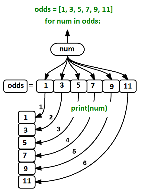
where each number (num) in the variable odds is looped through and printed one number after another. The other numbers in the diagram denote which loop cycle the number was printed in (1 being the first loop cycle, and 6 being the final loop cycle).

We can call the loop variable anything we like, but there must be a colon at the end of the line starting the loop, and we must indent anything we want to run inside the loop. Unlike many other languages, there is no command to signify the end of the loop body (e.g., end for); everything indented after the for statement belongs to the loop.

What’s in a name?

In the example above, the loop variable was given the name num as a mnemonic; it is short for ‘number’. We can choose any name we want for variables. We might just as easily have chosen the name banana for the loop variable, as long as we use the same name when we invoke the variable inside the loop:

PYTHON

odds = [1, 3, 5, 7, 9, 11]
for banana in odds:
   print(banana)

OUTPUT

1
3
5
7
9
11

It is a good idea to choose variable names that are meaningful, otherwise it would be more difficult to understand what the loop is doing.

Here’s another loop that repeatedly updates a variable:

PYTHON

length = 0
names = ['Curie', 'Darwin', 'Turing']
for value in names:
    length = length + 1
print('There are', length, 'names in the list.')

OUTPUT

There are 3 names in the list.

It’s worth tracing the execution of this little program step by step. Since there are three names in names, the statement on line 4 will be executed three times. The first time around, length is zero (the value assigned to it on line 1) and value is Curie. The statement adds 1 to the old value of length, producing 1, and updates length to refer to that new value. The next time around, value is Darwin and length is 1, so length is updated to be 2. After one more update, length is 3; since there is nothing left in names for Python to process, the loop finishes and the print function on line 5 tells us our final answer.

Note that a loop variable is a variable that is being used to record progress in a loop. It still exists after the loop is over, and we can re-use variables previously defined as loop variables as well:

PYTHON

name = 'Rosalind'
for name in ['Curie', 'Darwin', 'Turing']:
    print(name)
print('after the loop, name is', name)

OUTPUT

Curie
Darwin
Turing
after the loop, name is Turing

Note also that finding the length of an object is such a common operation that Python actually has a built-in function to do it called len:

PYTHON

print(len([0, 1, 2, 3]))

OUTPUT

4

len is much faster than any function we could write ourselves, and much easier to read than a two-line loop; it will also give us the length of many other data types we haven’t seen yet, so we should always use it when we can.

From 1 to N

Python has a built-in function called range that generates a sequence of numbers range can accept 1, 2, or 3 parameters.

• If one parameter is given, range generates a sequence of that length, starting at zero and incrementing by 1. For example, range(3) produces the numbers 0, 1, 2.
• If two parameters are given, range starts at the first and ends just before the second, incrementing by one. For example, range(2, 5) produces 2, 3, 4.
• If range is given 3 parameters, it starts at the first one, ends just before the second one, and increments by the third one. For example, range(3, 10, 2) produces 3, 5, 7, 9.

Using range, write a loop that uses range to print the first 3 natural numbers:

OUTPUT

1
2
3

Show me the solution

PYTHON

for number in range(1, 4):
   print(number)

Understanding the loops

Given the following loop:

PYTHON

word = 'oxygen'
for letter in word:
    print(letter)

How many times is the body of the loop executed?

• 3 times
• 4 times
• 5 times
• 6 times

Show me the solution

The body of the loop is executed 6 times.

Computing Powers With Loops

Exponentiation is built into Python:

PYTHON

print(5 ** 3)

OUTPUT

125

Write a loop that calculates the same result as 5 ** 3 using multiplication (and without exponentiation).

Show me the solution

PYTHON

result = 1
for number in range(0, 3):
    result = result * 5
print(result)

Summing a List

Write a loop that calculates the sum of elements in a list by adding each element and printing the final value, so [124, 402, 36] prints 562

Show me the solution

PYTHON

numbers = [124, 402, 36]
summed = 0
for num in numbers:
    summed = summed + num
print(summed)

Computing the Value of a Polynomial

The built-in function enumerate takes a sequence (e.g., a list) and generates a new sequence of the same length. Each element of the new sequence is a pair composed of the index (0, 1, 2,…) and the value from the original sequence:

PYTHON

for idx, val in enumerate(a_list):
    # Do something using idx and val

The code above loops through a_list, assigning the index to idx and the value to val.

Suppose you have encoded a polynomial as a list of coefficients in the following way: the first element is the constant term, the second element is the coefficient of the linear term, the third is the coefficient of the quadratic term, etc.

PYTHON

x = 5
coefs = [2, 4, 3]
y = coefs[0] * x**0 + coefs[1] * x**1 + coefs[2] * x**2
print(y)

OUTPUT

97

Write a loop using enumerate(coefs) which computes the value y of any polynomial, given x and coefs.

Show me the solution

PYTHON

y = 0
for idx, coef in enumerate(coefs):
    y = y + coef * x**idx

Making Choices with Conditional Logic

---

How can we use Python to automatically recognize different situations we encounter with our data and take a different action for each? In this lesson, we’ll learn how to write code that runs only when certain conditions are true.

Conditionals

We can ask Python to take different actions, depending on a condition, with an if statement:

PYTHON

num = 37
if num > 100:
    print('greater')
else:
    print('not greater')
print('done')

OUTPUT

not greater
done

The second line of this code uses the keyword if to tell Python that we want to make a choice. If the test that follows the if statement is true, the body of the if (i.e., the set of lines indented underneath it) is executed, and “greater” is printed. If the test is false, the body of the else is executed instead, and “not greater” is printed. Only one or the other is ever executed before continuing on with program execution to print “done”:

Conditional statements don’t have to include an else. If there isn’t one, Python simply does nothing if the test is false:

PYTHON

num = 53
print('before conditional...')
if num > 100:
    print(num, 'is greater than 100')
print('...after conditional')

OUTPUT

before conditional...
...after conditional

We can also chain several tests together using elif, which is short for “else if”. The following Python code uses elif to print the sign of a number.

PYTHON

num = -3

if num > 0:
    print(num, 'is positive')
elif num == 0:
    print(num, 'is zero')
else:
    print(num, 'is negative')

OUTPUT

-3 is negative

Note that to test for equality we use a double equals sign == rather than a single equals sign = which is used to assign values.

Comparing in Python

Along with the > and == operators we have already used for comparing values in our conditionals, there are a few more options to know about:

• >: greater than
• <: less than
• ==: equal to
• !=: does not equal
• >=: greater than or equal to
• <=: less than or equal to

We can also combine tests using and and or. and is only true if both parts are true:

PYTHON

if (1 > 0) and (-1 >= 0):
    print('both parts are true')
else:
    print('at least one part is false')

OUTPUT

at least one part is false

while or is true if at least one part is true:

PYTHON

if (1 < 0) or (1 >= 0):
    print('at least one test is true')

OUTPUT

at least one test is true

True and False

True and False are special words in Python called booleans, which represent truth values. A statement such as 1 < 0 returns the value False, while -1 < 0 returns the value True.

Checking Our Data

Now that we’ve seen how conditionals work, we can use them to check for the suspicious features we saw in our inflammation data. We are about to use functions provided by the numpy module again. Therefore, if you’re working in a new Python session, make sure to load the module with:

PYTHON

import numpy

From the first couple of plots, we saw that maximum daily inflammation exhibits a strange behavior and raises one unit a day. Wouldn’t it be a good idea to detect such behavior and report it as suspicious? Let’s do that! However, instead of checking every single day of the study, let’s merely check if maximum inflammation in the beginning (day 0) and in the middle (day 20) of the study are equal to the corresponding day numbers.

PYTHON

max_inflammation_0 = numpy.amax(data, axis=0)[0]
max_inflammation_20 = numpy.amax(data, axis=0)[20]

if max_inflammation_0 == 0 and max_inflammation_20 == 20:
    print('Suspicious looking maxima!')

We also saw a different problem in the third dataset; the minima per day were all zero (looks like a healthy person snuck into our study). We can also check for this with an elif condition:

PYTHON

elif numpy.sum(numpy.amin(data, axis=0)) == 0:
    print('Minima add up to zero!')

And if neither of these conditions are true, we can use else to give the all-clear:

PYTHON

else:
    print('Seems OK!')

Let’s test that out:

PYTHON

data = numpy.loadtxt(fname='inflammation-01.csv', delimiter=',')

max_inflammation_0 = numpy.amax(data, axis=0)[0]
max_inflammation_20 = numpy.amax(data, axis=0)[20]

if max_inflammation_0 == 0 and max_inflammation_20 == 20:
    print('Suspicious looking maxima!')
elif numpy.sum(numpy.amin(data, axis=0)) == 0:
    print('Minima add up to zero!')
else:
    print('Seems OK!')

OUTPUT

Suspicious looking maxima!

PYTHON

data = numpy.loadtxt(fname='inflammation-03.csv', delimiter=',')

max_inflammation_0 = numpy.amax(data, axis=0)[0]
max_inflammation_20 = numpy.amax(data, axis=0)[20]

if max_inflammation_0 == 0 and max_inflammation_20 == 20:
    print('Suspicious looking maxima!')
elif numpy.sum(numpy.amin(data, axis=0)) == 0:
    print('Minima add up to zero!')
else:
    print('Seems OK!')

OUTPUT

Minima add up to zero!

In this way, we have asked Python to do something different depending on the condition of our data. Here we printed messages in all cases, but we could also imagine not using the else catch-all so that messages are only printed when something is wrong, freeing us from having to manually examine every plot for features we’ve seen before.

How Many Paths?

Consider this code:

PYTHON

if 4 > 5:
    print('A')
elif 4 == 5:
    print('B')
elif 4 < 5:
    print('C')

Which of the following would be printed if you were to run this code? Why did you pick this answer?

1. A
2. B
3. C
4. B and C

Show me the solution

C gets printed because the first two conditions, 4 > 5 and 4 == 5, are not true, but 4 < 5 is true. In this case, only one of these conditions can be true for at a time, but in other scenarios multiple elif conditions could be met. In these scenarios, only the action associated with the first true elif condition will occur, starting from the top of the conditional section.

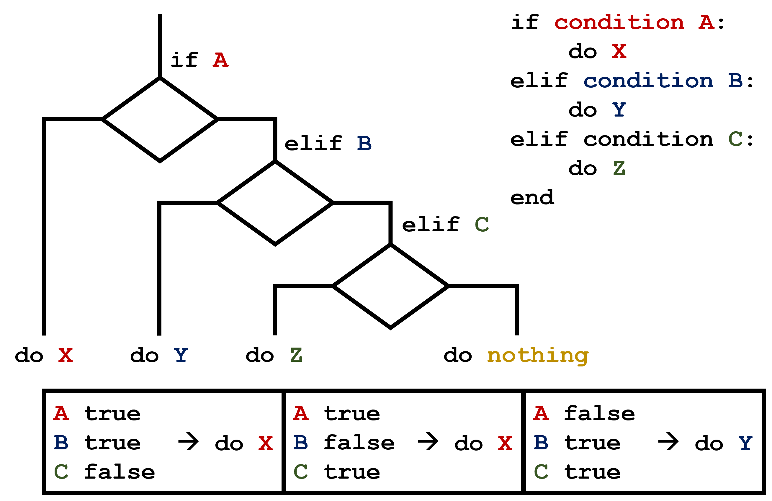
This contrasts with the case of multiple if statements, where every action can occur as long as their condition is met.

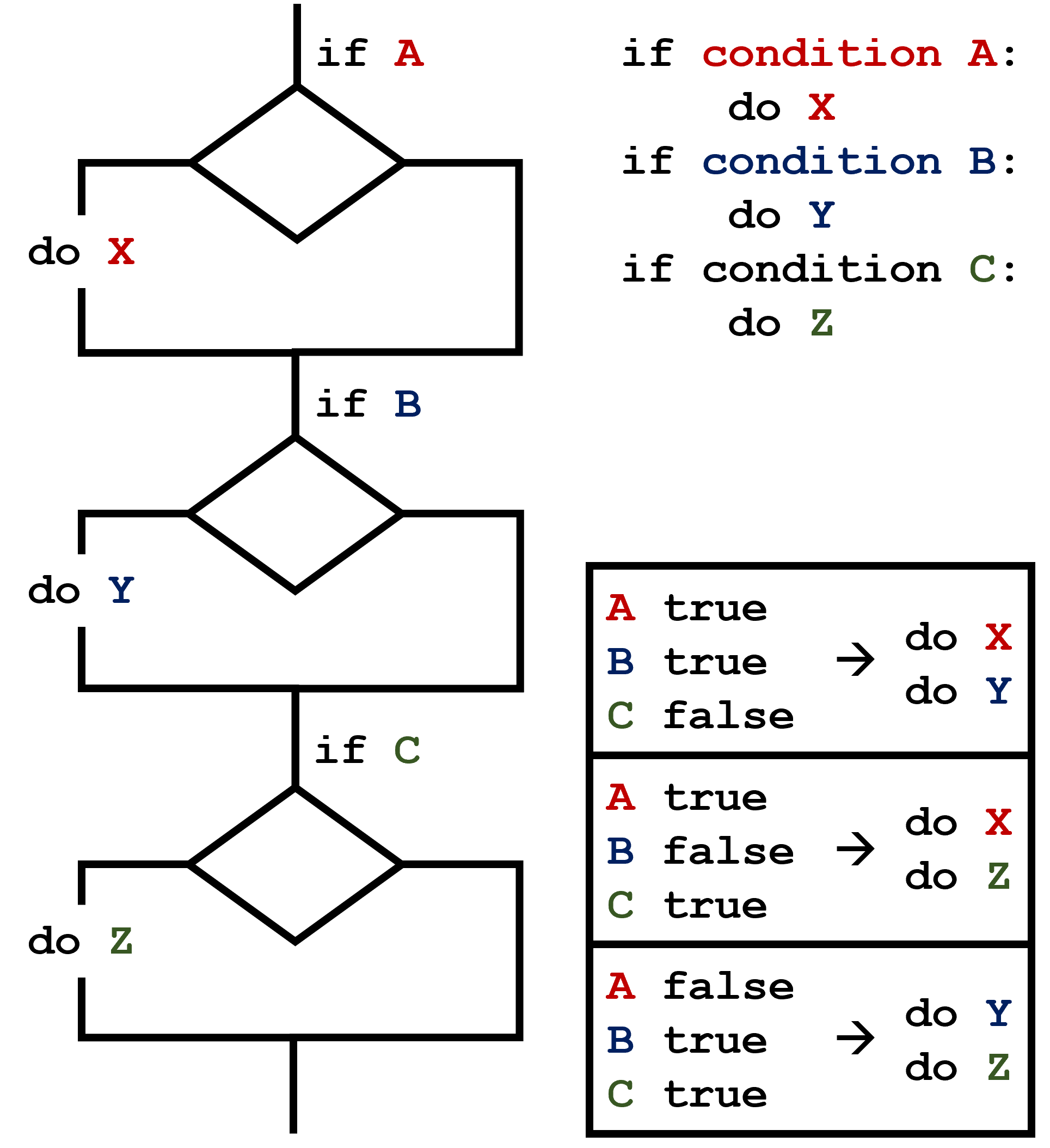
What Is Truth?

True and False booleans are not the only values in Python that are true and false. In fact, any value can be used in an if or elif. After reading and running the code below, explain what the rule is for which values are considered true and which are > considered false.

PYTHON

if '':
    print('empty string is true')
if 'word':
    print('word is true')
if []:
    print('empty list is true')
if [1, 2, 3]:
    print('non-empty list is true')
if 0:
    print('zero is true')
if 1:
    print('one is true')

That’s Not Not What I Meant

Sometimes it is useful to check whether some condition is not true. The Boolean operator not can do this explicitly. After reading and running the code below, write some if statements that use not to test the rule that you formulated in the previous challenge.

PYTHON

if not '':
    print('empty string is not true')
if not 'word':
    print('word is not true')
if not not True:
    print('not not True is true')

Close Enough

Write some conditions that print True if the variable a is within 10% of the variable b and False otherwise. Compare your implementation with your partner’s. Do you get the same answer for all possible pairs of numbers?

Hint

There is a built-in function abs that returns the absolute value of a number:

PYTHON

print(abs(-12))

OUTPUT

12

Solution 1

PYTHON

a = 5
b = 5.1

if abs(a - b) <= 0.1 * abs(b):
    print('True')
else:
    print('False')

Solution 2

PYTHON

print(abs(a - b) <= 0.1 * abs(b))

This works because the Booleans True and False have string representations which can be printed.

In-Place Operators

Python (and most other languages in the C family) provides in-place operators that work like this:

PYTHON

x = 1  # original value
x += 1 # add one to x, assigning result back to x
x *= 3 # multiply x by 3
print(x)

OUTPUT

6

Write some code that sums the positive and negative numbers in a list separately, using in-place operators. Do you think the result is more or less readable than writing the same without in-place operators?

Show me the solution

PYTHON

positive_sum = 0
negative_sum = 0
test_list = [3, 4, 6, 1, -1, -5, 0, 7, -8]
for num in test_list:
    if num > 0:
        positive_sum += num
    elif num == 0:
        pass
    else:
        negative_sum += num
print(positive_sum, negative_sum)

Here pass means “don’t do anything”. In this particular case, it’s not actually needed, since if num == 0 neither sum needs to change, but it illustrates the use of elif and pass.

Sorting a List Into Buckets

In our data folder, large data sets are stored in files whose names start with “inflammation-” and small data sets – in files whose names start with “small-”. We also have some other files that we do not care about at this point. We’d like to break all these files into three lists called large_files, small_files, and other_files, respectively.

Add code to the template below to do this. Note that the string method startswith returns True if and only if the string it is called on starts with the string passed as an argument, that is:

PYTHON

'String'.startswith('Str')

OUTPUT

True

But

PYTHON

'String'.startswith('str')

OUTPUT

False

Use the following Python code as your starting point:

PYTHON

filenames = ['inflammation-01.csv',
         'myscript.py',
         'inflammation-02.csv',
         'small-01.csv',
         'small-02.csv']
large_files = []
small_files = []
other_files = []

Your solution should:

1. loop over the names of the files
2. figure out which group each filename belongs in
3. append the filename to that list

In the end the three lists should be:

PYTHON

large_files = ['inflammation-01.csv', 'inflammation-02.csv']
small_files = ['small-01.csv', 'small-02.csv']
other_files = ['myscript.py']

Show me the solution

PYTHON

for filename in filenames:
    if filename.startswith('inflammation-'):
        large_files.append(filename)
    elif filename.startswith('small-'):
        small_files.append(filename)
    else:
        other_files.append(filename)

print('large_files:', large_files)
print('small_files:', small_files)
print('other_files:', other_files)

Counting Vowels

1. Write a loop that counts the number of vowels in a character string.
2. Test it on a few individual words and full sentences.
3. Once you are done, compare your solution to your neighbor’s. Did you make the same decisions about how to handle the letter ‘y’ (which some people think is a vowel, and some do not)?

Solution

vowels = 'aeiouAEIOU'
sentence = 'Mary had a little lamb.'
count = 0
for char in sentence:
   if char in vowels:
       count += 1

print('The number of vowels in this string is ' + str(count))

{.challenge}

Key Points

• Use for variable in sequence to process the elements of a sequence one at a time.
• The body of a for loop must be indented.
• Use len(thing) to determine the length of something that contains other values.
• Use if condition to start a conditional statement, elif condition to provide additional tests, and else to provide a default.
• The bodies of the branches of conditional statements must be indented.
• Use == to test for equality.
• X and Y is only true if both X and Y are true.
• X or Y is true if either X or Y, or both, are true.
• Zero, the empty string, and the empty list are considered false; all other numbers, strings, and lists are considered true.
• True and False represent truth values.

Content from Fetching data from APIs

---

Last updated on 2024-12-11 | Edit this page

Overview

Questions

• How to get data using a public API ?
• How to transform a JSON output to a panda dataframe ?
• Why the API documentation is essential to succeed in getting the expected data ?

Objectives

• Learn how to fetch data from an API using Python and load it into a Pandas DataFrame for analysis.

Prerequisites

• Basic understanding of Python (variables, functions, and loops).
• Python installed on your computer.
• Install the following libraries: requests and pandas:

BASH

pip install requests pandas

---

Steps

1. Import Required Libraries

To get started, import the necessary libraries:

PYTHON

import requests
import pandas as pd

2. Understand the API Endpoint

For this exercise, we will use the World Development Indicators (WDI) API from the World Bank. This API provides economic and development data for countries. An example endpoint is:

http://api.worldbank.org/v2/country/all/indicator/NY.GDP.MKTP.CD?format=json&date=2020:2021

This URL fetches GDP data (indicator NY.GDP.MKTP.CD) for all countries for the years 2020 and 2021.

3. Make an API Request

Use the requests library to fetch data from the API. Example:

PYTHON

url = "http://api.worldbank.org/v2/country/all/indicator/NY.GDP.MKTP.CD?format=json&date=2020:2021"
response = requests.get(url)
data = response.json()

• response.json() converts the API response into a Python dictionary or list.

4. Extract Relevant Data

Examine the JSON response structure. For example, the WDI API returns a list where the second element contains the actual data. Extract the relevant data for analysis:

PYTHON

# Extract data from JSON response
data_records = data[1]

# Prepare a list for DataFrame creation
data_list = []
for record in data_records:
    country = record["country"]["value"]
    year = record["date"]
    gdp_value = record["value"]
    data_list.append({
        "Country": country,
        "Year": int(year),
        "GDP": gdp_value
    })

5. Convert to DataFrame

Use the extracted data to create a Pandas DataFrame:

PYTHON

df = pd.DataFrame(data_list)
print(df.head())

6. Save or Analyze the Data

Save the DataFrame as a CSV file for later use:

PYTHON

df.to_csv("wdi_gdp_data.csv", index=False)

Or analyze the data directly using Pandas functions like:

PYTHON

print(df.describe())

---

Complete Example Code

PYTHON

import requests
import pandas as pd

# API Request
url = "http://api.worldbank.org/v2/country/all/indicator/NY.GDP.MKTP.CD?format=json&date=2020:2021"
response = requests.get(url)
data = response.json()

# Extract Data
data_records = data[1]
data_list = []
for record in data_records:
    country = record["country"]["value"]
    year = record["date"]
    gdp_value = record["value"]
    data_list.append({
        "Country": country,
        "Year": int(year),
        "GDP": gdp_value
    })

# Create DataFrame
df = pd.DataFrame(data_list)

# Save DataFrame
df.to_csv("wdi_gdp_data.csv", index=False)
print("Data saved to wdi_gdp_data.csv")

---

Key Takeaways

• Use requests to fetch API data.
• Convert JSON responses to a Pandas DataFrame.
• Save or analyze the data using Pandas.

Practice with the OECD Data Explorer to build confidence!

Practice with other APIs to build confidence!

• Let’s try with the OECD Data Explorer API

Content from Creating Functions

---

Last updated on 2024-12-10 | Edit this page

Overview

Questions

• What are functions, and how can I use them in Python?
• How can I define new functions?
• What’s the difference between defining and calling a function?
• What happens when I call a function?

Objectives

• identify what a function is
• create new functions
• Set default values for function parameters.
• Explain why we should divide programs into small, single-purpose functions.

At this point, we’ve seen that code can have Python make decisions about what it sees in our data. What if we want to convert some of our data, like taking a temperature in Fahrenheit and converting it to Celsius. We could write something like this for converting a single number

PYTHON

fahrenheit_val = 99
celsius_val = ((fahrenheit_val - 32) * (5/9))

and for a second number we could just copy the line and rename the variables

PYTHON

fahrenheit_val = 99
celsius_val = ((fahrenheit_val - 32) * (5/9))

fahrenheit_val2 = 43
celsius_val2 = ((fahrenheit_val2 - 32) * (5/9))

But we would be in trouble as soon as we had to do this more than a couple times. Cutting and pasting it is going to make our code get very long and very repetitive, very quickly. We’d like a way to package our code so that it is easier to reuse, a shorthand way of re-executing longer pieces of code. In Python we can use ‘functions’. Let’s start by defining a function fahr_to_celsius that converts temperatures from Fahrenheit to Celsius:

PYTHON

def explicit_fahr_to_celsius(temp):
    # Assign the converted value to a variable
    converted = ((temp - 32) * (5/9))
    # Return the value of the new variable
    return converted
    
def fahr_to_celsius(temp):
    # Return converted value more efficiently using the return
    # function without creating a new variable. This code does
    # the same thing as the previous function but it is more explicit
    # in explaining how the return command works.
    return ((temp - 32) * (5/9))

The function definition opens with the keyword def followed by the name of the function (fahr_to_celsius) and a parenthesized list of parameter names (temp). The body of the function — the statements that are executed when it runs — is indented below the definition line. The body concludes with a return keyword followed by the return value.

When we call the function, the values we pass to it are assigned to those variables so that we can use them inside the function. Inside the function, we use a return statement to send a result back to whoever asked for it.

Let’s try running our function.

PYTHON

fahr_to_celsius(32)

This command should call our function, using “32” as the input and return the function value.

In fact, calling our own function is no different from calling any other function:

PYTHON

print('freezing point of water:', fahr_to_celsius(32), 'C')
print('boiling point of water:', fahr_to_celsius(212), 'C')

OUTPUT

freezing point of water: 0.0 C
boiling point of water: 100.0 C

We’ve successfully called the function that we defined, and we have access to the value that we returned.

Composing Functions

---

Now that we’ve seen how to turn Fahrenheit into Celsius, we can also write the function to turn Celsius into Kelvin:

PYTHON

def celsius_to_kelvin(temp_c):
    return temp_c + 273.15

print('freezing point of water in Kelvin:', celsius_to_kelvin(0.))

OUTPUT

freezing point of water in Kelvin: 273.15

What about converting Fahrenheit to Kelvin? We could write out the formula, but we don’t need to. Instead, we can compose the two functions we have already created:

PYTHON

def fahr_to_kelvin(temp_f):
    temp_c = fahr_to_celsius(temp_f)
    temp_k = celsius_to_kelvin(temp_c)
    return temp_k

print('boiling point of water in Kelvin:', fahr_to_kelvin(212.0))

OUTPUT

boiling point of water in Kelvin: 373.15

This is our first taste of how larger programs are built: we define basic operations, then combine them in ever-larger chunks to get the effect we want. Real-life functions will usually be larger than the ones shown here — typically half a dozen to a few dozen lines — but they shouldn’t ever be much longer than that, or the next person who reads it won’t be able to understand what’s going on.

Variable Scope

---

In composing our temperature conversion functions, we created variables inside of those functions, temp, temp_c, temp_f, and temp_k. We refer to these variables as local variables because they no longer exist once the function is done executing. If we try to access their values outside of the function, we will encounter an error:

PYTHON

print('Again, temperature in Kelvin was:', temp_k)

ERROR

---------------------------------------------------------------------------
NameError                                 Traceback (most recent call last)
<ipython-input-1-eed2471d229b> in <module>
----> 1 print('Again, temperature in Kelvin was:', temp_k)

NameError: name 'temp_k' is not defined

If you want to reuse the temperature in Kelvin after you have calculated it with fahr_to_kelvin, you can store the result of the function call in a variable:

PYTHON

temp_kelvin = fahr_to_kelvin(212.0)
print('temperature in Kelvin was:', temp_kelvin)

OUTPUT

temperature in Kelvin was: 373.15

The variable temp_kelvin, being defined outside any function, is said to be global.

Inside a function, one can read the value of such global variables:

PYTHON

def print_temperatures():
  print('temperature in Fahrenheit was:', temp_fahr)
  print('temperature in Kelvin was:', temp_kelvin)

temp_fahr = 212.0
temp_kelvin = fahr_to_kelvin(temp_fahr)

print_temperatures()

OUTPUT

temperature in Fahrenheit was: 212.0
temperature in Kelvin was: 373.15

By giving our functions human-readable names, we can more easily read and understand what is happening in the for loop. Even better, if at some later date we want to use either of those pieces of code again, we can do so in a single line.

Testing and Documenting

---

Once we start putting things in functions so that we can re-use them, we need to start testing that those functions are working correctly. To see how to do this, let’s write a function to offset a dataset so that it’s mean value shifts to a user-defined value:

PYTHON

def offset_mean(data, target_mean_value):
    return (data - numpy.mean(data)) + target_mean_value

We could test this on our actual data, but since we don’t know what the values ought to be, it will be hard to tell if the result was correct. Instead, let’s use NumPy to create a matrix of 0’s and then offset its values to have a mean value of 3:

PYTHON

z = numpy.zeros((2,2))
print(offset_mean(z, 3))

OUTPUT

[[ 3.  3.]
 [ 3.  3.]]

That looks right, so let’s try offset_mean on our real data:

PYTHON

data = numpy.loadtxt(fname='inflammation-01.csv', delimiter=',')
print(offset_mean(data, 0))

OUTPUT

[[-6.14875 -6.14875 -5.14875 ... -3.14875 -6.14875 -6.14875]
 [-6.14875 -5.14875 -4.14875 ... -5.14875 -6.14875 -5.14875]
 [-6.14875 -5.14875 -5.14875 ... -4.14875 -5.14875 -5.14875]
 ...
 [-6.14875 -5.14875 -5.14875 ... -5.14875 -5.14875 -5.14875]
 [-6.14875 -6.14875 -6.14875 ... -6.14875 -4.14875 -6.14875]
 [-6.14875 -6.14875 -5.14875 ... -5.14875 -5.14875 -6.14875]]

It’s hard to tell from the default output whether the result is correct, but there are a few tests that we can run to reassure us:

PYTHON

print('original min, mean, and max are:', numpy.amin(data), numpy.mean(data), numpy.amax(data))
offset_data = offset_mean(data, 0)
print('min, mean, and max of offset data are:',
      numpy.amin(offset_data),
      numpy.mean(offset_data),
      numpy.amax(offset_data))

OUTPUT

original min, mean, and max are: 0.0 6.14875 20.0
min, mean, and and max of offset data are: -6.14875 2.84217094304e-16 13.85125

That seems almost right: the original mean was about 6.1, so the lower bound from zero is now about -6.1. The mean of the offset data isn’t quite zero — we’ll explore why not in the challenges — but it’s pretty close. We can even go further and check that the standard deviation hasn’t changed:

PYTHON

print('std dev before and after:', numpy.std(data), numpy.std(offset_data))

OUTPUT

std dev before and after: 4.61383319712 4.61383319712

Those values look the same, but we probably wouldn’t notice if they were different in the sixth decimal place. Let’s do this instead:

PYTHON

print('difference in standard deviations before and after:',
      numpy.std(data) - numpy.std(offset_data))

OUTPUT

difference in standard deviations before and after: -3.5527136788e-15

Again, the difference is very small. It’s still possible that our function is wrong, but it seems unlikely enough that we should probably get back to doing our analysis.

Documentation

---

We have one more task first, though: we should write some documentation for our function to remind ourselves later what it’s for and how to use it.

The usual way to put documentation in software is to add comments like this:

PYTHON

# offset_mean(data, target_mean_value):
# return a new array containing the original data with its mean offset to match the desired value.
def offset_mean(data, target_mean_value):
    return (data - numpy.mean(data)) + target_mean_value

There’s a better way, though. If the first thing in a function is a string that isn’t assigned to a variable, that string is attached to the function as its documentation:

PYTHON

def offset_mean(data, target_mean_value):
    """Return a new array containing the original data
       with its mean offset to match the desired value."""
    return (data - numpy.mean(data)) + target_mean_value

This is better because we can now ask Python’s built-in help system to show us the documentation for the function:

PYTHON

help(offset_mean)

OUTPUT

Help on function offset_mean in module __main__:

offset_mean(data, target_mean_value)
    Return a new array containing the original data with its mean offset to match the desired value.

A string like this is called a docstring. We don’t need to use triple quotes when we write one, but if we do, we can break the string across multiple lines:

PYTHON

def offset_mean(data, target_mean_value):
    """Return a new array containing the original data
       with its mean offset to match the desired value.

    Examples
    --------
    >>> offset_mean([1, 2, 3], 0)
    array([-1.,  0.,  1.])
    """
    return (data - numpy.mean(data)) + target_mean_value

help(offset_mean)

OUTPUT

Help on function offset_mean in module __main__:

offset_mean(data, target_mean_value)
    Return a new array containing the original data
       with its mean offset to match the desired value.

    Examples
    --------
    >>> offset_mean([1, 2, 3], 0)
    array([-1.,  0.,  1.])

Defining Defaults

---

We have passed parameters to functions in two ways: directly, as in type(data), and by name, as in numpy.loadtxt(fname='something.csv', delimiter=','). In fact, we can pass the filename to loadtxt without the fname=:

PYTHON

numpy.loadtxt('inflammation-01.csv', delimiter=',')

OUTPUT

array([[ 0.,  0.,  1., ...,  3.,  0.,  0.],
       [ 0.,  1.,  2., ...,  1.,  0.,  1.],
       [ 0.,  1.,  1., ...,  2.,  1.,  1.],
       ...,
       [ 0.,  1.,  1., ...,  1.,  1.,  1.],
       [ 0.,  0.,  0., ...,  0.,  2.,  0.],
       [ 0.,  0.,  1., ...,  1.,  1.,  0.]])

but we still need to say delimiter=:

PYTHON

numpy.loadtxt('inflammation-01.csv', ',')

ERROR

Traceback (most recent call last):
  File "<stdin>", line 1, in <module>
  File "/Users/username/anaconda3/lib/python3.6/site-packages/numpy/lib/npyio.py", line 1041, in loa
dtxt
    dtype = np.dtype(dtype)
  File "/Users/username/anaconda3/lib/python3.6/site-packages/numpy/core/_internal.py", line 199, in
_commastring
    newitem = (dtype, eval(repeats))
  File "<string>", line 1
    ,
    ^
SyntaxError: unexpected EOF while parsing

To understand what’s going on, and make our own functions easier to use, let’s re-define our offset_mean function like this:

PYTHON

def offset_mean(data, target_mean_value=0.0):
    """Return a new array containing the original data
       with its mean offset to match the desired value, (0 by default).

    Examples
    --------
    >>> offset_mean([1, 2, 3])
    array([-1.,  0.,  1.])
    """
    return (data - numpy.mean(data)) + target_mean_value

The key change is that the second parameter is now written target_mean_value=0.0 instead of just target_mean_value. If we call the function with two arguments, it works as it did before:

PYTHON

test_data = numpy.zeros((2, 2))
print(offset_mean(test_data, 3))

OUTPUT

[[ 3.  3.]
 [ 3.  3.]]

But we can also now call it with just one parameter, in which case target_mean_value is automatically assigned the default value of 0.0:

PYTHON

more_data = 5 + numpy.zeros((2, 2))
print('data before mean offset:')
print(more_data)
print('offset data:')
print(offset_mean(more_data))

OUTPUT

data before mean offset:
[[ 5.  5.]
 [ 5.  5.]]
offset data:
[[ 0.  0.]
 [ 0.  0.]]

This is handy: if we usually want a function to work one way, but occasionally need it to do something else, we can allow people to pass a parameter when they need to but provide a default to make the normal case easier. The example below shows how Python matches values to parameters:

PYTHON

def display(a=1, b=2, c=3):
    print('a:', a, 'b:', b, 'c:', c)

print('no parameters:')
display()
print('one parameter:')
display(55)
print('two parameters:')
display(55, 66)

OUTPUT

no parameters:
a: 1 b: 2 c: 3
one parameter:
a: 55 b: 2 c: 3
two parameters:
a: 55 b: 66 c: 3

As this example shows, parameters are matched up from left to right, and any that haven’t been given a value explicitly get their default value. We can override this behavior by naming the value as we pass it in:

PYTHON

print('only setting the value of c')
display(c=77)

OUTPUT

only setting the value of c
a: 1 b: 2 c: 77

With that in hand, let’s look at the help for numpy.loadtxt:

PYTHON

help(numpy.loadtxt)

OUTPUT

Help on function loadtxt in module numpy.lib.npyio:

loadtxt(fname, dtype=<class 'float'>, comments='#', delimiter=None, converters=None, skiprows=0, use
cols=None, unpack=False, ndmin=0, encoding='bytes')
    Load data from a text file.

    Each row in the text file must have the same number of values.

    Parameters
    ----------
...

There’s a lot of information here, but the most important part is the first couple of lines:

OUTPUT

loadtxt(fname, dtype=<class 'float'>, comments='#', delimiter=None, converters=None, skiprows=0, use
cols=None, unpack=False, ndmin=0, encoding='bytes')

This tells us that loadtxt has one parameter called fname that doesn’t have a default value, and eight others that do. If we call the function like this:

PYTHON

numpy.loadtxt('inflammation-01.csv', ',')

then the filename is assigned to fname (which is what we want), but the delimiter string ',' is assigned to dtype rather than delimiter, because dtype is the second parameter in the list. However ',' isn’t a known dtype so our code produced an error message when we tried to run it. When we call loadtxt we don’t have to provide fname= for the filename because it’s the first item in the list, but if we want the ',' to be assigned to the variable delimiter, we do have to provide delimiter= for the second parameter since delimiter is not the second parameter in the list.

Readable functions

---

Consider these two functions:

PYTHON

def s(p):
    a = 0
    for v in p:
        a += v
    m = a / len(p)
    d = 0
    for v in p:
        d += (v - m) * (v - m)
    return numpy.sqrt(d / (len(p) - 1))

def std_dev(sample):
    sample_sum = 0
    for value in sample:
        sample_sum += value

    sample_mean = sample_sum / len(sample)

    sum_squared_devs = 0
    for value in sample:
        sum_squared_devs += (value - sample_mean) * (value - sample_mean)

    return numpy.sqrt(sum_squared_devs / (len(sample) - 1))

The functions s and std_dev are computationally equivalent (they both calculate the sample standard deviation), but to a human reader, they look very different. You probably found std_dev much easier to read and understand than s.

As this example illustrates, both documentation and a programmer’s coding style combine to determine how easy it is for others to read and understand the programmer’s code. Choosing meaningful variable names and using blank spaces to break the code into logical “chunks” are helpful techniques for producing readable code. This is useful not only for sharing code with others, but also for the original programmer. If you need to revisit code that you wrote months ago and haven’t thought about since then, you will appreciate the value of readable code!

Combining Strings

“Adding” two strings produces their concatenation: 'a' + 'b' is 'ab'. Write a function called fence that takes two parameters called original and wrapper and returns a new string that has the wrapper character at the beginning and end of the original. A call to your function should look like this:

PYTHON

print(fence('name', '*'))

OUTPUT

*name*

Show me the solution

PYTHON

def fence(original, wrapper):
    return wrapper + original + wrapper

Return versus print

Note that return and print are not interchangeable. print is a Python function that prints data to the screen. It enables us, users, see the data. return statement, on the other hand, makes data visible to the program. Let’s have a look at the following function:

PYTHON

def add(a, b):
    print(a + b)

Question: What will we see if we execute the following commands?

PYTHON

A = add(7, 3)
print(A)

Show me the solution

Python will first execute the function add with a = 7 and b = 3, and, therefore, print 10. However, because function add does not have a line that starts with return (no return “statement”), it will, by default, return nothing which, in Python world, is called None. Therefore, A will be assigned to None and the last line (print(A)) will print None. As a result, we will see:

OUTPUT

10
None

Selecting Characters From Strings

If the variable s refers to a string, then s[0] is the string’s first character and s[-1] is its last. Write a function called outer that returns a string made up of just the first and last characters of its input. A call to your function should look like this:

PYTHON

print(outer('helium'))

OUTPUT

hm

Show me the solution

PYTHON

def outer(input_string):
    return input_string[0] + input_string[-1]

Rescaling an Array

Write a function rescale that takes an array as input and returns a corresponding array of values scaled to lie in the range 0.0 to 1.0. (Hint: If L and H are the lowest and highest values in the original array, then the replacement for a value v should be (v-L) / (H-L).)

Show me the solution

PYTHON

def rescale(input_array):
    L = numpy.amin(input_array)
    H = numpy.amax(input_array)
    output_array = (input_array - L) / (H - L)
    return output_array

Testing and Documenting Your Function

Run the commands help(numpy.arange) and help(numpy.linspace) to see how to use these functions to generate regularly-spaced values, then use those values to test your rescale function. Once you’ve successfully tested your function, add a docstring that explains what it does.

Show me the solution

PYTHON

"""Takes an array as input, and returns a corresponding array scaled so
that 0 corresponds to the minimum and 1 to the maximum value of the input array.

Examples:
>>> rescale(numpy.arange(10.0))
array([ 0.        ,  0.11111111,  0.22222222,  0.33333333,  0.44444444,
       0.55555556,  0.66666667,  0.77777778,  0.88888889,  1.        ])
>>> rescale(numpy.linspace(0, 100, 5))
array([ 0.  ,  0.25,  0.5 ,  0.75,  1.  ])
"""

Defining Defaults

Rewrite the rescale function so that it scales data to lie between 0.0 and 1.0 by default, but will allow the caller to specify lower and upper bounds if they want. Compare your implementation to your neighbor’s: do the two functions always behave the same way?

Show me the solution

PYTHON

def rescale(input_array, low_val=0.0, high_val=1.0):
    """rescales input array values to lie between low_val and high_val"""
    L = numpy.amin(input_array)
    H = numpy.amax(input_array)
    intermed_array = (input_array - L) / (H - L)
    output_array = intermed_array * (high_val - low_val) + low_val
    return output_array

Variables Inside and Outside Functions

What does the following piece of code display when run — and why?

PYTHON

f = 0
k = 0

def f2k(f):
    k = ((f - 32) * (5.0 / 9.0)) + 273.15
    return k

print(f2k(8))
print(f2k(41))
print(f2k(32))

print(k)

Show me the solution

OUTPUT

259.81666666666666
278.15
273.15
0

k is 0 because the k inside the function f2k doesn’t know about the k defined outside the function. When the f2k function is called, it creates a local variable k. The function does not return any values and does not alter k outside of its local copy. Therefore the original value of k remains unchanged. Beware that a local k is created because f2k internal statements affect a new value to it. If k was only read, it would simply retrieve the global k value.

Mixing Default and Non-Default Parameters

Given the following code:

PYTHON

def numbers(one, two=2, three, four=4):
    n = str(one) + str(two) + str(three) + str(four)
    return n

print(numbers(1, three=3))

what do you expect will be printed? What is actually printed? What rule do you think Python is following?

1. 1234
2. one2three4
3. 1239
4. SyntaxError

Given that, what does the following piece of code display when run?

PYTHON

def func(a, b=3, c=6):
    print('a: ', a, 'b: ', b, 'c:', c)

func(-1, 2)

1. a: b: 3 c: 6
2. a: -1 b: 3 c: 6
3. a: -1 b: 2 c: 6
4. a: b: -1 c: 2

Show me the solution

Attempting to define the numbers function results in 4. SyntaxError. The defined parameters two and four are given default values. Because one and three are not given default values, they are required to be included as arguments when the function is called and must be placed before any parameters that have default values in the function definition.

The given call to func displays a: -1 b: 2 c: 6. -1 is assigned to the first parameter a, 2 is assigned to the next parameter b, and c is not passed a value, so it uses its default value 6.

Readable Code

Revise a function you wrote for one of the previous exercises to try to make the code more readable. Then, collaborate with one of your neighbors to critique each other’s functions and discuss how your function implementations could be further improved to make them more readable.

Key Points

• Define a function using def function_name(parameter).
• The body of a function must be indented.
• Call a function using function_name(value).
• Numbers are stored as integers or floating-point numbers.
• Variables defined within a function can only be seen and used within the body of the function.
• Variables created outside of any function are called global variables.
• Within a function, we can access global variables.
• Variables created within a function override global variables if their names match.
• Use help(thing) to view help for something.
• Put docstrings in functions to provide help for that function.
• Specify default values for parameters when defining a function using name=value in the parameter list.
• Parameters can be passed by matching based on name, by position, or by omitting them (in which case the default value is used).
• Put code whose parameters change frequently in a function, then call it with different parameter values to customize its behavior.

Content from Errors and Exceptions

---

Last updated on 2024-12-10 | Edit this page

Overview

Questions

• How does Python report errors?
• How can I handle errors in Python programs?

Objectives

• identify different errors and correct bugs associated with them

Every programmer encounters errors, both those who are just beginning, and those who have been programming for years. Encountering errors and exceptions can be very frustrating at times, and can make coding feel like a hopeless endeavour. However, understanding what the different types of errors are and when you are likely to encounter them can help a lot. Once you know why you get certain types of errors, they become much easier to fix.

Errors in Python have a very specific form, called a traceback. Let’s examine one:

PYTHON

# This code has an intentional error. You can type it directly or
# use it for reference to understand the error message below.
def favorite_ice_cream():
    ice_creams = [
        'chocolate',
        'vanilla',
        'strawberry'
    ]
    print(ice_creams[3])

favorite_ice_cream()

ERROR

---------------------------------------------------------------------------
IndexError                                Traceback (most recent call last)
<ipython-input-1-70bd89baa4df> in <module>()
      9     print(ice_creams[3])
      10
----> 11 favorite_ice_cream()

<ipython-input-1-70bd89baa4df> in favorite_ice_cream()
      7         'strawberry'
      8     ]
----> 9     print(ice_creams[3])
      10
      11 favorite_ice_cream()

IndexError: list index out of range

This particular traceback has two levels. You can determine the number of levels by looking for the number of arrows on the left hand side. In this case:

1. The first shows code from the cell above, with an arrow pointing to Line 11 (which is favorite_ice_cream()).

2. The second shows some code in the function favorite_ice_cream, with an arrow pointing to Line 9 (which is print(ice_creams[3])).

The last level is the actual place where the error occurred. The other level(s) show what function the program executed to get to the next level down. So, in this case, the program first performed a function call to the function favorite_ice_cream. Inside this function, the program encountered an error on Line 6, when it tried to run the code print(ice_creams[3]).

Long Tracebacks

Sometimes, you might see a traceback that is very long -- sometimes they might even be 20 levels deep! This can make it seem like something horrible happened, but the length of the error message does not reflect severity, rather, it indicates that your program called many functions before it encountered the error. Most of the time, the actual place where the error occurred is at the bottom-most level, so you can skip down the traceback to the bottom.

So what error did the program actually encounter? In the last line of the traceback, Python helpfully tells us the category or type of error (in this case, it is an IndexError) and a more detailed error message (in this case, it says “list index out of range”).

If you encounter an error and don’t know what it means, it is still important to read the traceback closely. That way, if you fix the error, but encounter a new one, you can tell that the error changed. Additionally, sometimes knowing where the error occurred is enough to fix it, even if you don’t entirely understand the message.

If you do encounter an error you don’t recognize, try looking at the official documentation on errors. However, note that you may not always be able to find the error there, as it is possible to create custom errors. In that case, hopefully the custom error message is informative enough to help you figure out what went wrong. Libraries like pandas and numpy have these custom errors, but the procedure to figure them out is the same: go to the earliest line in the error, and look at the error message for it. The documentation for these libraries will often provide the information you need about any functions you are using. There are also large communities of users for data libraries that can help as well!

Reading Error Messages

Read the Python code and the resulting traceback below, and answer the following questions:

1. How many levels does the traceback have?
2. What is the function name where the error occurred?
3. On which line number in this function did the error occur?
4. What is the type of error?
5. What is the error message?

PYTHON

# This code has an intentional error. Do not type it directly;
# use it for reference to understand the error message below.
def print_message(day):
    messages = [
        'Hello, world!',
        'Today is Tuesday!',
        'It is the middle of the week.',
        'Today is Donnerstag in German!',
        'Last day of the week!',
        'Hooray for the weekend!',
        'Aw, the weekend is almost over.'
    ]
    print(messages[day])

def print_sunday_message():
    print_message(7)

print_sunday_message()

ERROR

---------------------------------------------------------------------------
IndexError                                Traceback (most recent call last)
<ipython-input-7-3ad455d81842> in <module>
     16     print_message(7)
     17
---> 18 print_sunday_message()
     19

<ipython-input-7-3ad455d81842> in print_sunday_message()
     14
     15 def print_sunday_message():
---> 16     print_message(7)
     17
     18 print_sunday_message()

<ipython-input-7-3ad455d81842> in print_message(day)
     11         'Aw, the weekend is almost over.'
     12     ]
---> 13     print(messages[day])
     14
     15 def print_sunday_message():

IndexError: list index out of range

Show me the solution

1. 3 levels
2. print_message
3. 13
4. IndexError
5. list index out of range You can then infer that 7 is not the right index to use with messages.

Better errors on newer Pythons

Newer versions of Python have improved error printouts. If you are debugging errors, it is often helpful to use the latest Python version, even if you support older versions of Python.

Type Errors

---

One of the most common types of errors in Python are called type errors. These errors occur when you try to perform an operation on an object in python that cannot support it. This happens easily when working with large datasets where there are expected value types like either strings or integers. When we write a function expecting integers, we will not get an error until we encounter an operation that cannot handle strings. For example:

PYTHON

def our_function()
  my_string="Hello World"
  letter=my_string["e""]

ERROR

  File "<ipython-input-3-6bb841ea1423>", line 3
    letter=my_string["e"]
                       ^
TypeError: string indices must be integers

We get this error because we are trying to use an index to access part of our string, which requires an integer. Instead, we entered a character and received a type error. This is fixed by replacing “e” with 2.

In the case of datasets, we often see type errors when a mathematical operation, such as taking a mean, is performed on a column that contains characters, either as a result of formatting or introduced through error. As a result, correcting the error can involve simply removing the characters from the strings using regular expressions, or if the characters have resulted in incorrect data, removing those observations from the dataset.

Syntax Errors

---

When you forget a colon at the end of a line, accidentally add one space too many when indenting under an if statement, or forget a parenthesis, you will encounter a syntax error. This means that Python couldn’t figure out how to read your program. This is similar to forgetting punctuation in English: for example, this text is difficult to read there is no punctuation there is also no capitalization why is this hard because you have to figure out where each sentence ends you also have to figure out where each sentence begins to some extent it might be ambiguous if there should be a sentence break or not

People can typically figure out what is meant by text with no punctuation, but people are much smarter than computers. If Python doesn’t know how to read the program, it will give up and inform you with an error. For example:

PYTHON

def some_function()
    msg = 'hello, world!'
    print(msg)
     return msg

ERROR

  File "<ipython-input-3-6bb841ea1423>", line 1
    def some_function()
                       ^
SyntaxError: invalid syntax

Here, Python tells us that there is a SyntaxError on line 1, and even puts a little arrow in the place where there is an issue. In this case the problem is that the function definition is missing a colon at the end.

Actually, the function above has two issues with syntax. If we fix the problem with the colon, we see that there is also an IndentationError, which means that the lines in the function definition do not all have the same indentation:

PYTHON

def some_function():
    msg = 'hello, world!'
    print(msg)
     return msg

ERROR

  File "<ipython-input-4-ae290e7659cb>", line 4
    return msg
    ^
IndentationError: unexpected indent

Both SyntaxError and IndentationError indicate a problem with the syntax of your program, but an IndentationError is more specific: it always means that there is a problem with how your code is indented.

Tabs and Spaces

Some indentation errors are harder to spot than others. In particular, mixing spaces and tabs can be difficult to spot because they are both whitespace. In the example below, the first two lines in the body of the function some_function are indented with tabs, while the third line — with spaces. If you’re working in a Jupyter notebook, be sure to copy and paste this example rather than trying to type it in manually because Jupyter automatically replaces tabs with spaces.

PYTHON

def some_function():
	msg = 'hello, world!'
	print(msg)
        return msg

Visually it is impossible to spot the error. Fortunately, Python does not allow you to mix tabs and spaces.

ERROR

  File "<ipython-input-5-653b36fbcd41>", line 4
    return msg
              ^
TabError: inconsistent use of tabs and spaces in indentation

Variable Name Errors

---

Another very common type of error is called a NameError, and occurs when you try to use a variable that does not exist. For example:

PYTHON

print(a)

ERROR

---------------------------------------------------------------------------
NameError                                 Traceback (most recent call last)
<ipython-input-7-9d7b17ad5387> in <module>()
----> 1 print(a)

NameError: name 'a' is not defined

Variable name errors come with some of the most informative error messages, which are usually of the form “name ‘the_variable_name’ is not defined”.

Why does this error message occur? That’s a harder question to answer, because it depends on what your code is supposed to do. However, there are a few very common reasons why you might have an undefined variable. The first is that you meant to use a string, but forgot to put quotes around it:

PYTHON

print(hello)

ERROR

---------------------------------------------------------------------------
NameError                                 Traceback (most recent call last)
<ipython-input-8-9553ee03b645> in <module>()
----> 1 print(hello)

NameError: name 'hello' is not defined

The second reason is that you might be trying to use a variable that does not yet exist. In the following example, count should have been defined (e.g., with count = 0) before the for loop:

PYTHON

for number in range(10):
    count = count + number
print('The count is:', count)

ERROR

---------------------------------------------------------------------------
NameError                                 Traceback (most recent call last)
<ipython-input-9-dd6a12d7ca5c> in <module>()
      1 for number in range(10):
----> 2     count = count + number
      3 print('The count is:', count)

NameError: name 'count' is not defined

Finally, the third possibility is that you made a typo when you were writing your code. Let’s say we fixed the error above by adding the line Count = 0 before the for loop. Frustratingly, this actually does not fix the error. Remember that variables are case-sensitive, so the variable count is different from Count. We still get the same error, because we still have not defined count:

PYTHON

Count = 0
for number in range(10):
    count = count + number
print('The count is:', count)

ERROR

---------------------------------------------------------------------------
NameError                                 Traceback (most recent call last)
<ipython-input-10-d77d40059aea> in <module>()
      1 Count = 0
      2 for number in range(10):
----> 3     count = count + number
      4 print('The count is:', count)

NameError: name 'count' is not defined

Index Errors

---

Next up are errors having to do with containers (like lists and strings) and the items within them. If you try to access an item in a list or a string that does not exist, then you will get an error. This makes sense: if you asked someone what day they would like to get coffee, and they answered “caturday”, you might be a bit annoyed. Python gets similarly annoyed if you try to ask it for an item that doesn’t exist:

PYTHON

letters = ['a', 'b', 'c']
print('Letter #1 is', letters[0])
print('Letter #2 is', letters[1])
print('Letter #3 is', letters[2])
print('Letter #4 is', letters[3])

OUTPUT

Letter #1 is a
Letter #2 is b
Letter #3 is c

ERROR

---------------------------------------------------------------------------
IndexError                                Traceback (most recent call last)
<ipython-input-11-d817f55b7d6c> in <module>()
      3 print('Letter #2 is', letters[1])
      4 print('Letter #3 is', letters[2])
----> 5 print('Letter #4 is', letters[3])

IndexError: list index out of range

Here, Python is telling us that there is an IndexError in our code, meaning we tried to access a list index that did not exist.

File Errors

---

The last type of error we’ll cover today are the most common type of error when using Python with data, those associated with reading and writing files: FileNotFoundError. If you try to read a file that does not exist, you will receive a FileNotFoundError telling you so. If you attempt to write to a file that was opened read-only, Python 3 returns an UnsupportedOperationError. More generally, problems with input and output manifest as OSErrors, which may show up as a more specific subclass; you can see the list in the Python docs. They all have a unique UNIX errno, which is you can see in the error message.

PYTHON

file_handle = open('myfile.txt', 'r')

ERROR

---------------------------------------------------------------------------
FileNotFoundError                         Traceback (most recent call last)
<ipython-input-14-f6e1ac4aee96> in <module>()
----> 1 file_handle = open('myfile.txt', 'r')

FileNotFoundError: [Errno 2] No such file or directory: 'myfile.txt'

One reason for receiving this error is that you specified an incorrect path to the file. For example, if I am currently in a folder called myproject, and I have a file in myproject/writing/myfile.txt, but I try to open myfile.txt, this will fail. The correct path would be writing/myfile.txt. It is also possible that the file name or its path contains a typo. There may also be specific settings based on your organization if you are using shared, networked, or cloud-based drives. It is best to check with your IT administrators if you are still encountering issues reading in a file after troubleshooting.

A related issue can occur if you use the “read” flag instead of the “write” flag. Python will not give you an error if you try to open a file for writing when the file does not exist. However, if you meant to open a file for reading, but accidentally opened it for writing, and then try to read from it, you will get an UnsupportedOperation error telling you that the file was not opened for reading:

PYTHON

file_handle = open('myfile.txt', 'w')
file_handle.read()

ERROR

---------------------------------------------------------------------------
UnsupportedOperation                      Traceback (most recent call last)
<ipython-input-15-b846479bc61f> in <module>()
      1 file_handle = open('myfile.txt', 'w')
----> 2 file_handle.read()

UnsupportedOperation: not readable

If you are getting a read or write error on file or folder that you are able to open and/or edit with other programs, you may need to contact an IT administrator to check the permissions granted to you and any programs you are using.

These are the most common errors with files, though many others exist. If you get an error that you’ve never seen before, searching the Internet for that error type often reveals common reasons why you might get that error.

Identifying Syntax Errors

1. Read the code below, and (without running it) try to identify what the errors are.
2. Run the code, and read the error message. Is it a SyntaxError or an IndentationError?
3. Fix the error.
4. Repeat steps 2 and 3, until you have fixed all the errors.

PYTHON

def another_function
  print('Syntax errors are annoying.')
   print('But at least Python tells us about them!')
  print('So they are usually not too hard to fix.')

Show me the solution

SyntaxError for missing (): at end of first line, IndentationError for mismatch between second and third lines. A fixed version is:

PYTHON

def another_function():
    print('Syntax errors are annoying.')
    print('But at least Python tells us about them!')
    print('So they are usually not too hard to fix.')

Identifying Variable Name Errors

1. Read the code below, and (without running it) try to identify what the errors are.
2. Run the code, and read the error message. What type of NameError do you think this is? In other words, is it a string with no quotes, a misspelled variable, or a variable that should have been defined but was not?
3. Fix the error.
4. Repeat steps 2 and 3, until you have fixed all the errors.

PYTHON

for number in range(10):
    # use a if the number is a multiple of 3, otherwise use b
    if (Number % 3) == 0:
        message = message + a
    else:
        message = message + 'b'
print(message)

Show me the solution

3 NameErrors for number being misspelled, for message not defined, and for a not being in quotes.

Fixed version:

PYTHON

message = ''
for number in range(10):
    # use a if the number is a multiple of 3, otherwise use b
    if (number % 3) == 0:
        message = message + 'a'
    else:
        message = message + 'b'
print(message)

Identifying Index Errors

1. Read the code below, and (without running it) try to identify what the errors are.
2. Run the code, and read the error message. What type of error is it?
3. Fix the error.

PYTHON

seasons = ['Spring', 'Summer', 'Fall', 'Winter']
print('My favorite season is ', seasons[4])

Show me the solution

IndexError; the last entry is seasons[3], so seasons[4] doesn’t make sense. A fixed version is:

PYTHON

seasons = ['Spring', 'Summer', 'Fall', 'Winter']
print('My favorite season is ', seasons[-1])

A Final Note About Correcting Errors

---

There are a lot of very helpful answers for many error messages, however when working with official statistics, we need to also exercise some caution. Be aware and be wary of any answers that ask you to download a package from someone’s personal GitHub repository or other file sharing service. Try to find the type of error first and understand what the issue is before downloading anything claiming to fix the error. If the error is the result of an issue with a version of a package, check if there are any security vulnerabilities with that version, and use a package manager to move between package versions.

Key Points

• NULL